CEGS 2017 Workshop: RNA-Seq Differential Expression Analysis
Document originally produced by Chet Birger and Marc-Danie Nazaire (2014). Updated by Sara Garamszegi (2017).
The computational workflow supporting the differential expression (DE) analysis of RNA-Seq data typically consists of several high-level steps; GenePattern supports modules for conducting each of these steps. Today’s exercise makes use of GenomeSpace, GenePattern and IGV. The steps necessary to complete today’s DE analysis of RNA-Seq data are illustrated below:

Slides for this workshop can be found on the public GenomeSpace user account, SharedData, by navigating to the following folder: Public > SharedData > Presentations > CEGS_2017-01-31.
Data used in this exercise:
This exercise recapitulates and extends (employing gene set enrichment analysis) some of the findings in the following paper by Himes et al. (2014), "RNA-Seq Transcriptome Profiling Identifies CRISPLD2 as a Glucocorticoid Responsive Gene that Modulates Cytokine Function in Airway Smooth Muscle Cells". The authors, using an in vitro model, employed RNA-Seq to comprehensively characterize changes in the transcriptome of airway smooth muscle (ASM) cells in response to treatment with Glucocorticoids (GCs), a common class of medications used to treat inflammatory diseases, including asthma. One of the goals of the study was to increase understanding of how GCs work in ASM cells to alleviate asthma symptoms.
Paper methods:
Sample collection:
ASM cells were isolated and cultured from lung tissue of four donors. Total RNA was extracted from control and treated ASM cells from each donor culture, yielding 8 total samples, 4 untreated and 4 treated. Treatment consisted of exposure to dexamethasone, a synthetic glucocorticoid (1 for 18 hours).
Sequencing:
Sequencing of 75 bp paired-end reads was performed with an Illumina HiSeq 2000 instrument at the Partners HealthCare Center for Personalized Genetic Medicine (Boston, MA). Preliminary processing of raw reads was performed using Casava 1.8 (Illumina, Inc., San Diego, CA).
Data from the study is publicly available from NCBI/GEO/SRA: http://www.ncbi.nlm.nih.gov/geo/query/acc.cgi?acc=GSE52778
Data preprocessing:
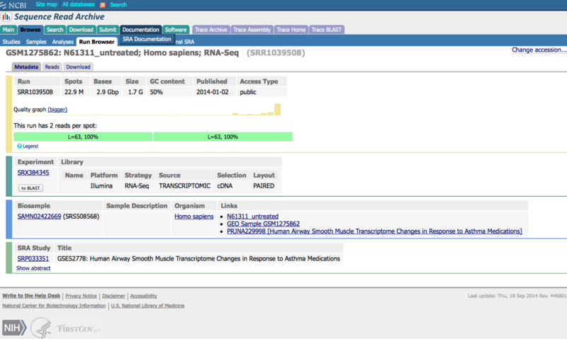
The data the authors posted to NCBI/SRA had already undergone some preliminary trimming. Using the FastQC tool to obtain QC metrics, the authors observed sequence bias in the initial 12 bases on the 5’ ends of reads. The first 12 bases of all reads were trimmed (using the FASTX toolkit), and the trimmed data was submitted to SRA. Thus, the reported read length is 63 bp rather than 75 bp.
Below is the entry in NCBI’s Sequence Read Archive (SRA) for one of the untreated samples, which illustrates the difference in read length:
Description of samples:
| SRA run accession |
Donor ID |
Phenotype |
Base Read Count (Gbp) |
| SRR1039508 |
N061311 |
untreated |
2.9 |
| SRR1039509 |
N061311 |
dex |
2.7 |
| SRR1039512 |
N052611 |
untreated |
3.5 |
| SRR1039513 |
N052611 |
dex |
3.8 |
| SRR1039516 |
N080611 |
untreated |
3.6 |
| SRR1039517 |
N080611 |
dex |
4.3 |
| SRR1039520 |
N061011 |
untreated |
3.5 |
| SRR1039521 |
N061011 |
dex |
4.1 |
Re-creating the workflow
This document contains detailed instructions on how to run through each step in the computational workflow. The GenePattern part of the computational workflow has been previously run on the public GenePattern server. Public read access has been granted to all these jobs and links have been provided for accessing each of these completed jobs, e.g.,
http://bit.ly/ZxbsqV: job status page for TopHat alignment job on sample SRR1039508
Enter the link in your browser’s address bar (make sure you have already logged into the public GenePattern server), and the job status page from the previously run job will appear, e.g.,
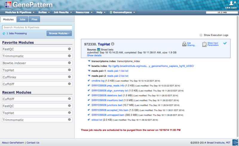
To re-run a GenePattern job from its job status page, click on the module name (e.g., TopHat), and a slide-out menu will appear. Clicking on the Reload Job selection from that menu will allow you to re-run that job.
Since we are working with the complete dataset from an actual study, the processing time required to run through the workflow (hours) far exceeds the time allotted to us in the workshop. We will be examining the results of the previously run jobs. You may re-run this workflow, outside of the workshop, by following the detailed instructions below.
STEP 1: Retrieve the FASTQ files from GenomeSpace
We begin by downloading the raw sequence data. This data was originally obtained by using GenePattern’s SraToFastQ module to retrieve the RNA-Seq read data from NCBI’s Sequence Read Archive (SRA) website, and converting it from the compressed SRA format to the FASTQ format. However, in this exercise we provide the converted, paired FASTQ files on a GenomeSpace public folder for users. Each sample has two gzipped files. For example, sample SRR1039508 has files SRR1039508_1.fastq.gz, and SRR1039508_2.fastq.gz.
Steps:
- Go to GenomeSpace (http://gsui.genomespace.org).
- Navigate to the following folder: Home/Public/SharedData/Presentations/CEGS_Oct 1_2015/Data (http://bit.ly/1FuJAaP)
- We will use the data in this folder to run jobs in GenePattern in the next step.
Links to the files on GenomeSpace (NOTE: clicking the links will begin downloading the files!):
STEP 2: Run FastQC on all pairs of FASTQ files
We will run quality control checks on each of the FASTQ files before alignment. We utilize a GenePattern module that runs the FastQC quality control tool for high-throughput sequence data (Babraham Institute, 2012). This tool detects irregularities in the short reads data and generates a report that guides subsequent data trimming and filtering. Typically, one would run the FastQC module on each RNA-Seq reads input file. For paired-end experiments, each mate of a pair of read files undergoes FastQC analysis separately. We will use GenePattern’s batch feature to launch two FastQC jobs per sample, one for each of the two mated read files.
Steps:
- Go to the GenePattern main page (http://cloud.genepattern.org)
- Select the Modules tab, and search for “FastQC”
- Select FastQC
- Select the Files tab, then navigate to the public GenomeSpace folder containing the FASTQ files: Home/Public/SharedData/Presentations/CEGS_Oct 1_2015/Data
- Change the following parameters:
- Under Basic:
- input file: check “batch”
- Drag two paired fastq.gz files to the parameter’s input box.
For example, for sample SRR1039508, use files SRR1039508_1.fastq.gz and SRR1039508_2.fastq.gz
- Click Run. This will launch two FastQC jobs, one for each fastq.gz file.
For example, for sample SRR1039508, this will generate the following two outputs:
- http://bit.ly/ZCOLSq: job status page for FastQC job on SRR1039508_1.fastq.gz
- http://bit.ly/1sV4KlI: job status page for FastQC job on SRR1039508_2.fastq.gz
The approximate run time is 10 minutes for each job (20 minutes per sample).
- Repeat Steps 1-5 for the remaining 7 samples.
Below is an example output from running FastQC, for the sample SRR1039508_1.fastq.gz:
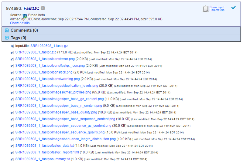
Links to the job status pages for runs of FastQC on all eight samples:
View results:
To view the results of the job, click on any of the …fastqc/fastqc_report.html output files. For example, to view the results for the first mate in the paired sample SRR1039508, click on the file, SRR1039508_1_fastqc/fastqc_report.html. A menu will slide out. Select Open Link to open the FastQC report in a new tab.
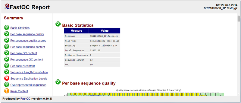
Below is the FastQC report generated from running the module on SRR109508_1.fastq.gz:
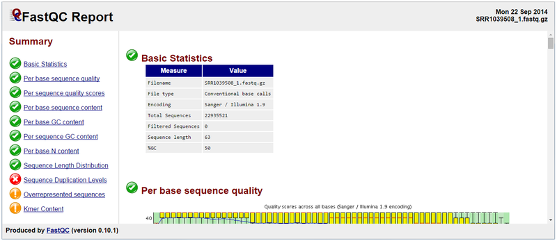
Three areas are flagged as requiring some level of review: Sequence Duplication Levels, Overrepresented sequences and Kmer Content.
An error flag is raised for Sequence Duplication Levels if non-unique sequences make up more than 50% of the total number of reads. A warning or error flag in this FastQC module is simply a statement that you have exhausted the diversity in at least part of your library and are re-sequencing the same sequences repeatedly. Sequences from different transcripts will be present at a wide range of different levels in the starting population. In order to be able to observe lowly expressed transcripts it is therefore common to greatly over-sequence highly expressed transcripts, leading to large sets of duplicates. Thus moderate to high levels of duplication may indicate a very high level of coverage of highly expressed transcripts. A high level of duplication may also indicate some kind of enrichment bias (e.g., PCR over-amplification).
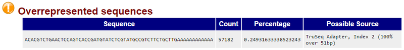
The Overrepresented sequences report indicates the presence of a contaminant TruSeq adapter sequence at relatively high level. Contaminant sequences may be removed using GenePattern’s Trimmomatic module (see STEP 3). An example of an overrepresented sequence from a contaminating TruSeq adapter is shown below:
Reviewing the FastQC reports for all 16 fastq files (two per sample) shows that a handful of the fastq files have evidence of adapter contamination, and most have reports of sequence duplication levels at the warning or error levels. Most of the fastq files were also flagged at the warning level for Kmer content.
In the next step we will run the Trimmomatic module on each sample’s reads to eliminate contaminant sequences.
STEP 3: Remove contaminant sequences and re-evaluate quality
STEP 3.1: Run Trimmomatic on all paired FASTQ files
Here, we will run GenePattern’s Trimmomatic module on each sample’s paired end reads. The module directly exposes through its GUI six of the most frequently used trimming/filtering operations on raw RNA-Seq data. These are:
- Trimming Illumina Adapters
- Trimming Leading Low-quality Base Reads
- Trimming Trailing Low-quality Base Reads
- Sliding Window Quality Trimming
- Adaptive Quality Trimming
- Minimum-length Read Filtering
We will enable Trimming Illumina Adapters and Minimum-length Read Filtering. Short reads are more likely to align to multiple sites on a reference genome, and thus provide ambiguous information. After adapter clipping operations have been completed, you should filter the reads so that they all satisfy a specific minimum length. To enable read length filtering, set the min read length parameter. In this exercise, we set the min read length parameter to 50 bp. After completing the trimming operation, we re-run FastQC on the trimmed forward reads for sample SRR1039508 (i.e. SRR1039508_1.fastq.gz) and observe the elimination of the contaminating TruSeq adapter sequences.
Steps:
- Go to the GenePattern main page (http://cloud.genepattern.org)
- Select the Modules tab, and search for “Trimmomatic”
- Select Trimmomatic
- Change the following parameters:
- Under Basic Input Parameters and Options:
- input file 1: drag the first of the mated read files generated from a run of SraToFastQ to the parameter’s input box. For example, sample SRR1039508, would be SRR1039508_1.fastq.gz.
- input file 2: drag the second of the mated read files generated from a run of SraToFastQ to the parameter’s input box. For example, sample SRR1039508, would be SRR1039508_2.fastq.gz.
- Under Adapter Clipping:
- adapter clip sequence file: TruSeq2-PE.fa
- adapter clip seed mismatches: 2
- adapter clip palindrome clip threshold: 40
- adapter clip simple clip threshold: 15
- Under Min Read Length:
- min read length: 50
- Click Run. This will launch one Trimmomatic job per sample.
The approximate run time is 15 minutes for each job.
- Repeat Steps 1-4 for the remaining 7 samples.
Links to the job status pages for runs of Trimmomatic on all eight samples:
For paired-end input, Trimmomatic creates four FASTQ output files:
- Two for the paired output where both reads of a pairing survived the trimming/filtering step. Denoted with a _#P in the filename, where # is either 1 or 2.
- Two for the leftover unpaired output containing unmatched reads where only one of the two paired reads survived trimming/filtering. Denoted with a _#U in the filename, where # is either 1 or 2.
For paired-end inputs, it is Trimmomatic’s paired output files (containing _#P in their names) that should undergo read alignment. For example, for sample SRR1039508, the SRR1039508_1P.fastq.gz and SRR1039508_2P.fastq.gz files would be further analyzed.
STEP 3.2: Re-run FastQC on paired FASTQ files
Once the trimming and filtering steps are completed, we can run the FastQC module on the Trimmomatic output files to observe the elimination of contaminant adapter sequences. For example, we can run SRR1039508_1P.fastq.gz and look at resulting fastqc_report.html.
Steps:
- Go to the GenePattern main page (http://cloud.genepattern.org)
- Select the Modules tab, and search for “FastQC”
- Select FastQC
- Change the following parameters:
- Under Basic:
- input file: drag the trimmed fastq.gz files generated from a run of Trimmomatic to the parameter’s input box
For example, sample SRR1039508, would use SRR1039508_1P.fastq.gz.
- Click Run. The approximate run time is 10 minutes for each job.
- Repeat Steps 1-5 for any remaining samples which were trimmed and had adapter sequences removed.
View results:
To view the results of the job, click on the …fastqc/fastqc_report.html output file. For example, for the trimmed sample SRR1039508_1P, the file is SRR1039508_1P_fastqc/fastqc_report.html. A menu will slide out, select Open Link to open the FastQC report in a new tab.
Below is the FastQC report generated from running the module on SRR109508_1P.fastq.gz:
We can see that the Overrepresented sequences section is no longer flagged as having issues. You can see the full FastQC report for sample SRR1039508_1P at the following link:
http://bit.ly/1p61J0P: job status page for FastQC job on SRR1039508_1P.fastq.gz
Note: TopHat’s alignment engine (Bowtie) takes into account base read quality scores when aligning reads. Thus, if using TopHat, there is no need to conduct quality base trimming before aligning the reads.
STEP 4: Run TopHat to align reads to a reference transcriptome
TopHat is an alignment algorithm using the Bowtie alignment engine. It is typically run in one of the following three modes:
- Alignment to the genome only
No genome annotation file (GTF) is provided, and the short sequence reads will be aligned directly to the reference genome. The optional GTF file and transcriptome index parameters are left blank. The quantification step requires a genome annotation; thus when aligning to the genome, it will be necessary to assemble the transcripts from the aligned reads and generate a GTF file specifying the assembled transcripts.
- Annotation-assisted alignment to the genome
If a genome annotation is available, but is believed to be incomplete, TopHat may be configured to use the incomplete annotation to assist the alignment to the genome. TopHat will extract the transcript sequences from the provided annotation and use Bowtie to directly align the reads to the known transcripts. Unmapped reads will be aligned to the genome. This mode requires either a genome annotation file (the GTF file parameter) or a transcriptome index (the transcriptome index parameter). As with genome-only alignment, annotation-assisted alignment requires transcript assembly.
- Alignment to the transcriptome only
If a high-quality reference annotation is available, the short sequence reads can be mapped directly to the known transcript sequences. TopHat will extract the transcript sequences from the provided annotation and use Bowtie to directly align the reads to the known transcripts. However, TopHat will not attempt to align unmapped reads to the transcriptome; unmapped reads are dropped from the analysis. This is the least computationally intensive mode of TopHat alignment. This mode requires either a genome annotation file (the GTF file parameter) or a transcriptome index (the transcriptome index parameter) and set the transcriptome only input option to yes.
TopHat records read alignments to a BAM (binary version of SAM) formatted file. It attaches a score to each alignment. This alignment score takes into account the read quality scores captured in the input FASTQ files as well as mismatches and indels.
In this exercise, we will align to the known transcript sequences only (Mode #3), relying on the UCSC hg19 reference annotation.
We must provide TopHat with either a genome annotation file (the GTF file parameter) or a transcriptome index (the transcriptome index parameter). If we provide a GTF file, TopHat builds a transcriptome sequence and a corresponding Bowtie index. Creating the Bowtie index for the transcriptome can be time-consuming. TopHat allows the reuse of a previously created transcriptome index to avoid its costly regeneration in each TopHat run. An initial run of TopHat can be made whose sole purpose is the creation of the transcriptome index: the bowtie index and GTF file parameters should be set, but the transcriptome index and read pairs parameters left blank. In subsequent runs, the directory containing the generated transcriptome index can be provided via the transcriptome index parameter.
STEP 4.1: Create a transcriptome index
First, we run TopHat to generate a transcriptome index for UCSC’s hg19 reference annotation, which we will use in subsequent TopHat runs to align each sample’s trimmed reads to the reference transcriptome.
Steps:
- Go to the GenePattern main page (http://cloud.genepattern.org)
- Select the Modules tab, and search for “TopHat”
- Select TopHat
- Change the following parameters:
- Under Basic Parameters:
- Bowtie index: Homo_sapiens_hg19_UCSC
- GTF file: Homo_sapiens_hg19_UCSC.gtf
- Click Run. The approximate run time is 20 minutes.
The result of this job will be a new Bowtie reference transcriptome index for UCSC’s hg19 reference annotation. The result of the job can be found at the following link:
http://bit.ly/1BTrDwL: job status page for TopHat job generating a trancriptome index
STEP 4.2: Align reads to a transcriptome
Steps:
- Go to the GenePattern main page (http://cloud.genepattern.org)
- Select the Modules tab, and search for “TopHat”
- Select TopHat
- Change the following parameters:
- Under Basic Parameters:
- Bowtie index: Homo_sapiens_hg19_UCSC
- Transcriptome index
- Click Add Path or URL…
- Set the Enter URL to: http://genepattern.broadinstitute.org/gp/jobResults/972317/transcriptome_index/
- reads pair 1: drag the first paired read file output from Trimmomatic to the input box. For example, use file SRR1039508_1P.fastq.gz.
- reads pair 2: drag the second paired read file output from Trimmomatic to the input box. For example, use file SRR1039508_2P.fastq.gz.
- library type: Standard Illumina (fr-unstranded)
- output prefix: SRR1039508
- Under Parameters Relevant when Transcriptome Search is Activated:
- transcriptome only: yes
- Click Run. The approximate run time is 1 hour 15 minutes.
- Repeat steps 1-5 on the remaining 7 samples. Make sure to personalize the output prefix parameter for each sample. If Trimmomatic was not run on a sample, then use the _1.fastq.gz file and _2.fastq.gz files for reads pair 1 and reads pair 2 instead.
Links to the job status pages for runs of TopHat on all eight samples:
STEP 5: Run CuffDiff to summarize and quantitate aligned reads, normalize expression estimates, and conduct differential expression analysis
The goal of summarization/quantitation is to accurately derive gene and transcript expression values from the aligned reads and a genome annotation. The annotation may have been constructed from the aligned reads or be an externally generated reference annotation. In the summarization/quantitation step, reads are assigned to the annotation’s transcripts that are most likely to have served as the transcription template for the sequenced cDNA.
Summarization/quantitation is not a simplistic accounting of the number of reads that map to each feature. Early methods for quantitating gene expression from RNA-Seq data counted the reads that mapped to the exons of each gene and divided each count by a scaling factor that was based on the total length of a gene’s exons. These “raw count” methods were shown to be less accurate than “isoform deconvolution” methods that estimate the expression levels of a gene’s alternative isoforms (transcripts) and then sum those transcript-level estimates to derive gene-level expression estimates.
Estimating transcript-level expression levels is complicated by the fact that a gene’s multiple isoforms often share exons and hence there is uncertainty in assigning a read to a specific isoform if the read maps to a shared exon. In other words, splicing structure introduces uncertainty that must be accounted for when deriving expression estimates from mapped reads. Many eukaryotic genes have multiple isoforms that share exons, leading to uncertainty around the assignment of a read to a particular transcript.
Normalization of the expression estimates permits accurate comparisons of features’ (transcripts or genes) expression levels within a single sample, and comparison of a single feature’s expression across different samples (phenotypes or conditions).
Following summarization/quantitation and normalization, differences in estimated transcript and gene expression levels across conditions can be analyzed. Differences in a feature’s estimated expression values across two conditions will be impacted by both true differences in expression levels and the inherent noise in the experimental data. Sources of experimental variability include sampling variance, technical variance, and biological variance. In addition to these three sources of experimental variance, RNA-Seq expression estimates are also subject to variability resulting from read assignment uncertainties. If there is a lot of similarity between a gene’s isoforms (e.g., shared exons) there will be a great deal of uncertainty attached to the expression estimates for each of those isoforms, which in turn will lead to uncertainty in the gene-level expression estimates.
Thus, differential expression analysis of RNA-Seq data requires the modeling of both experimental variation and read assignment uncertainty in order to assess the statistical significance of any observed difference in a transcript’s or gene’s expression levels across two conditions. In other words ,without a means of accurately assessing the amount of variability and uncertainty present in a feature’s expression estimates, one cannot determine whether observed differences in that feature’s expression levels across two conditions is the result of true differential expression, or an artifact of the inherent noise in the underlying expression estimates. Differential expression analysis tools, like Cuffdiff, calculate a variance for each transcript’s or gene’s expression estimates and uses that variance to estimate the variance of whatever statistic is employed to measure differential expression, e.g., log-fold change.
By conducting both quantification and differential analysis, Cuffdiff takes into account the uncertainty of mapping reads to isoforms when calculating variances of transcript-level expression estimates. This leads to more accurate assessments of the statistical significances of the observed changes in expression levels across conditions.
Steps:
- Go to the GenePattern main page (http://cloud.genepattern.org)
- Select the Modules tab, and search for “Cuffdiff”
- Select Cuffdiff
- Change the following parameters:
- Under Basic Parameters and Options:
- aligned files
- Set condition to untreated
- For each of the untreated samples (SRR1039508, SRR1039512, SRR1039516, SRR1039520), drag the TopHat output file SRR10395XX.accepted_hits.bam to the drag target
- Click Add Another Condition
- Set condition to dex
- For each of the dexamethasone-treated samples (SRR1039509, SRR1039513, SRR1039517, SRR1039521), drag the TopHat output file SRR10395XX.accepted_hits.bam to the drag target.
- GTF file: Homo_sapiens_hg19_UCSC.gtf
- frag bias correct: Homo_sapiens_hg19_UCSC.fa
- library type: fr-unstranded
- Click Run. The approximate run time is 6 hours.
This job will create one output representing the comparison of untreated and dexamethasone-treated samples, for all 8 samples:
http://bit.ly/1poBEt9: job status page for Cuffdiff job.
STEP 6: Run CummeRbund.QcReport to identify the top differentially expressed genes
CummeRbund is an R/Bioconductor package that supports analysis and visualization of the data produced by the Cuffdiff tool, both the expression datasets coming out of the quantitation and normalization steps and the test results from Cuffdiff’s differential expression analysis.
GenePattern supports four modules that utilize the CummeRbund package, which creates sets of plots and visualizations to better understand experimental results.
- CummeRbund.QcReport: creates high-level visualizations, allowing for comparisons across all conditions and all genes
- CummeRbund.GeneSetReport: creates visualizations focusing on a specific list of genes
- CummeRbund.SelectedGeneReport: creates visualizations focusing on a single user-chosen gene
- CummeRbund.SelectedConditionsReport: creates visualizations across all genes, but limited to a specific set of conditions
In this exercise, we will use the CummeRbund.QcReport module to obtain global statistics and plots, and to identify the top differentially expressed genes, based on specific thresholds and cut-off values. In particular, this module lists those genes that CuffDiff found to be differentially expressed with a Q-value (FDR) less than the specified FDR threshold, which by default is set to 0.05. These files can be found in the output file, QC_sig_diffExp_genes.txt (see below).
Steps:
- Go to the GenePattern main page (http://cloud.genepattern.org)
- Select the Modules tab, and search for “CummeRbund.QcReport”
- Select CummeRbund.QcReport
- Change the following parameters:
- cuffdiff input: drag the Cuffdiff job from the Jobs tab into the parameter input field.
- Click Run. The approximate run time is 5 minutes.
This job will create one output representing the comparison of untreated and dexamethasone-treated samples, for all 8 samples:
http://bit.ly/1uz8Vpt: job status page for CummeRbund.QcReport job
STEP 7: Visualize aligned reads and gene expression using IGV
Finally, we are interested in visualizing the results of our alignment. To do this, we will use the Integrative Genomics Viewer (IGV), a high-performance visualization tool for interactive exploration of large, integrated genomic datasets (Robinson et al. 2011). It supports a wide variety of data types, including array-based and next-generation sequence data, and genomic annotations.
We will load data into IGV directly from GenomeSpace, and visualize three sets of data:
- Genes.fpkm_tracking (http://bit.ly/1LQ1dPj): this is a result from the Cuffdiff job (Step 5), which contains estimated gene-level expression values in the Fragments Per Kilobase of transcript per Million mapped reads (FPKM) tracking format. This file contains expression information for both phenotypes (untreated vs. dex).
- SRR1039508.accepted_hits.sorted.bam (http://bit.ly/1NWlJnb): this file contains the accepted hits from a TopHat alignment on an untreated sample. This sample is from the same patient as SRR1039509. The reads have been aligned to the UCSC hg19 transcriptome. This file is also accompanied by a BAM index (.bai) file.
- SRR1039509.accepted_hits.sorted.bam (http://bit.ly/1JrKfVr): this file contains the accepted hits from a TopHat alignment on a dex-treated sample. This sample is from the same patient as SRR1039508. The reads have been aligned to the UCSC hg19 transcriptome. This file is also accompanied by a BAM index (.bai) file.
Steps:
- Go to GenomeSpace (http://gsui.genomespace.org).
- Click the IGV icon to launch IGV.
- A igv.jnlp file will be downloaded. Double-click the file to start IGV.
- You may receive a security warning; please ignore it.
- Once IGV is loaded, make sure that the Human (hg19) genome is selected.
- Load the above datasets into IGV by completing the following steps:
- Navigate to the following menu: GenomeSpace/Load File from GenomeSpace…
- In the file menu, navigate to the following folder: Public/SharedData/Presentations/CEGS_Oct 1_2015/Data
- Select genes.fpkm_tracking, then click “Open” to load the file.
NOTE: the tracks loaded in genes.fpkm_tracking may look mostly empty. This is due to an issue with scaling the data. To properly visualize the results, use ctrl+click to select both the genes.fpkm_tracking q00 and genes.fpkm_tracking q01 tracks, then right-click and select “log scale” to re-scale this data.
- Repeat Step 4 two more times to load the SRR1039508.accepted_hits.sorted.bam and SRR1039509.accepted_hits.sorted.bam files.
Viewing results:
We can now explore in IGV and visualize our results. You should see something that looks similar to the image below:
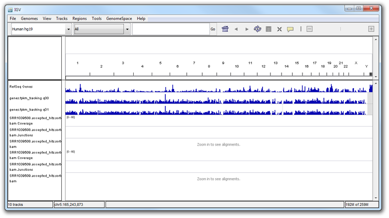
Here, we have a genome-level view of our results. To look at gene-specific results, you can enter the name of a gene in the search bar. From our results, we know that certain genes are differentially expressed when comparing the untreated and dex-treated phenotypes. We predict that these genes may have interesting patterns of aligned reads or expression.
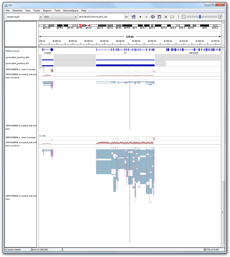
Try searching for some of the following genes in IGV: C7, CCDC69, DUSP1, FKBP5, GPX3, KLF15, MAOA, SAMHD1, SERPINA3, SPARCL3, TSC22D3, CRISPLD2, C13orf15, PER1, KCTD12, ERRFI1, STEAP4.
For an example, see the expression profile of the gene C7. Here, we see that there is higher expression in C7 in the dex phenotype (q01) than the untreated phenotype (q00). If we look at some BAM files representing these phenotypes, we similarly observe that there are fewer reads aligned against this gene in the untreated phenotype (SRR1039508) than the dex-treated phenotype (SRR1039509). The difference in the number of reads aligning to the gene location complements the difference observed in the gene-level expression profile of the untreated and dex-treated phenotypes.

 GenomeSpace.org