This is an example interpretation of the results from this recipe.
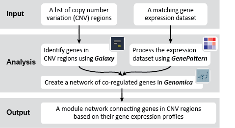
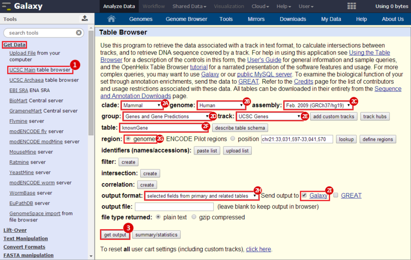
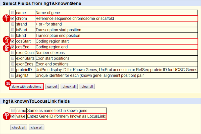
First, we identified the overlap between reference gene annotations (Entrez ID format) and the aberrant regions in cancer cells, using Galaxy. This resulted in a list of annotated genes that are located in the aberrant regions associated with cancer. In this example, we find roughly ~650 genes. Independently, we processed and normalized the microarray dataset so that the expression of genes associated with the aberrant regions could be observed. In this example, the microarray has roughly ~4000 genes. Using Genomica, we view the expression of the genes identified in aberrant regions, and try to find modules of similarly regulated genes, based on the list of candidate regulator genes from Galaxy. There are roughly ~100 genes which Galaxy identified which were also in the microarray; these ~100 genes are our 'candidate regulator genes'.
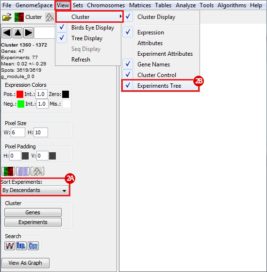
To view the regulatory program of a specific module, click on a part of the cluster heatmap and then use the triangle button in the left-side menu to view up-stream regulators of expression. In this example, we view one of the clusters and observe the regulatory program:
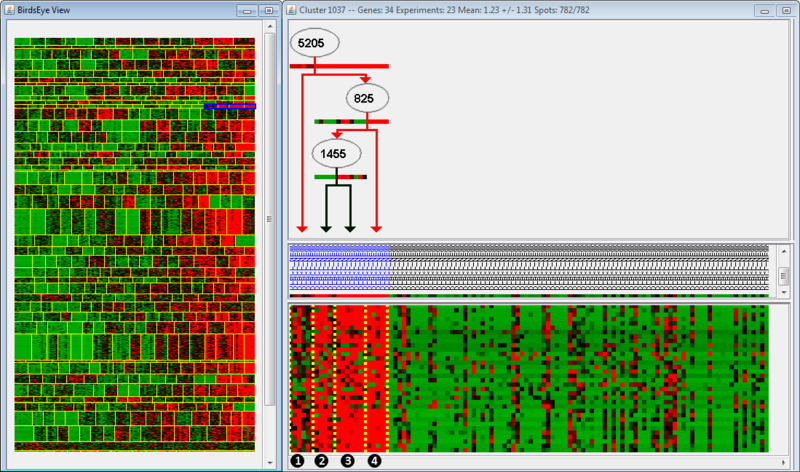
In the left panel is the BirdsEye view, which displays all the modules found by the algorithm. Each module is separated by horizontal yellow lines, and the splits within a module are separated by vertical yellow lines. Splits indicate that regulation of an up-stream gene changes from one group of arrays to the next. In this example, the module we are examining is highlighted in blue; note that only one part of the module is highlighted (we are examining only a few splits within the module). The right panel is the Cluster view of the microarray, organized according to the BirdsEye view. For example, the clusters we are examining (highlighted in blue) have been moved to the left side of the Cluster view, even though they are the rightmost clusters in the BirdsEye view. The top part of the second panel indicates the gene regulation program; the middle indicates the arrays grouped according to expression, and the bottom indicates the actual expression itself (as a microarray).
The regulation program illustrates which genes are thought to be associated with the regulation observed in the microarrays. Gene names are displayed along arrows indicating how the gene is regulated in different modules. Arrays are sorted to the left and right of the split by a boolean answer to the question, "Is GeneA up-regulated?" Arrays which are up-regulated for a gene will fall on the righthand side; all other arrays fall on the lefthand side. Let's examine the regulation program more closely. We see that Gene 5205 is up-regulated in Groups 2, 3, and 4, but not in Group 1. Gene 825 is up-regulated in Group 4, but not Groups 2 and 3. Finally, Gene 1455 is up-regulated in Group 3, but not 2. Therefore, we could say that Group 2 is associated with up-regulation of Gene 5205, but no up-regulation of Genes 825 or 1455.
However, the results in this example are just one interpretation and are only a simple representation of possible results.

 GenomeSpace.org


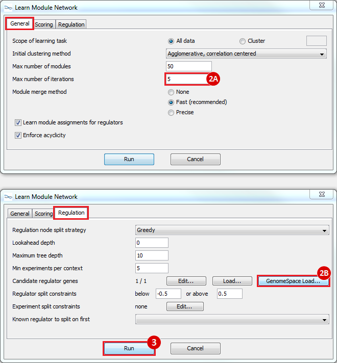
 to run
Hi everyone I have some trouble in “10: Loading files into Genomica “. When I launched Genomica and wanted to “Open From GenomeSpace” new window does not appear to choose "mrna_orig.preprocessed.gct" file form it. Can anyone help me please?