Galaxy igv

Identify and validate coding variants from exome sequencing data

Added by GenomeSpaceTeam on 2015.05.19 Official logo
Last updated on over 3 years ago.


Summary

What coding variants do my exome sequences contain, and are any of them phenotypically interesting?

This recipe provides a method to identify coding variants from exome sequencing data. An example use of this recipe is a case where an investigator may want to identify variants from their alignment data and evaluate the phenotypes.


In particular, this recipe uses the variant detector, FreeBayes, in Galaxy to identify potential variants from short-read alignments and assign them quality scores. We also use other Galaxy tools to pare these potential variants down to a high quality subset and to compare them against a catalog of gold-standard variants. Finally, we use IGV to visualize these variants alongside known pathogenic variants.

Why identify genetic variants? Genetic variants are DNA sequence differences that occur with relative frequency in a population. These variants include single nucleotide polymorphisms (SNPs), insertions and deletions (indels), multi-nucleotide polymorphisms (MNPs), and complex events that are combinations of indels and polymorphisms. With the advent of next generation sequencing technologies, it has become common practice to identify variants using sequence data. This is usually accomplished by comparing sequence data from many samples or individuals against a reference. Identified variants can have many practical applications. For instance, variants that correlate strongly with disease risk may provide insight into the disease's genetic underpinnings. Variants may also be used as biomarkers for disease risk or to DNA "fingerprint" individuals.

Why use exome sequencing data? The human exome comprises all the exonic regions of the human genome. That is, it includes all the DNA sequences that, after transcription into RNA, remain after RNA-splicing, which amounts to about 1% of the entire genome. Whole exome sequencing (WES) thus generates much less data than whole genome sequencing (WGS). Furthermore, since WES focuses almost exclusively on protein-coding regions it is an effective method for identifying coding variants.

NOTE: Working with DNA sequencing data is a computationally and resource intensive process. Files containing raw sequence reads can be many gigabytes in size and can be cumbersome to manage. To maintain the usability of this recipe, we have chosen to work with only a partial region of the human genome, specifically the exonic regions of a chromosome 20.

Inputs

To complete this recipe, we will need a number of datasets of various types. First, we will need a set of exonic sequence reads that have been pre-processed for quality and duplicates and aligned to the genome. In this example, we will use aligned reads generated by the 1000 Genomes Project that have been mapped to the exonic regions of chromosome 20. These samples are derived from 10 individuals in the project's Great Britain population cohort. We also require a reference genome in FASTA format, which we will use to identify variants. Finally, we will need a set of gold-standard variants as well as a set of variant annotations to compare against our discovered variants. We will need the following datasets, which can be downloaded from the following GenomeSpace Public folder:

Public > RecipeData > AlignmentData > 1000GP.GBR.chrom20.exome.tar.gz: This is an archive of aligned, sorted, and duplicate-marked chromosome 20 exome reads in BAM format. Specifically, the archive includes the alignments of 10 individuals drawn from the Great Britain population in Phase 3 of the 1000 Genome Project.

Public > RecipeData > SequenceData > hs_ref_GRCh37.p5_chr20.fa: This is a FASTA file containing sequences for a human reference genome, chromosome 20 only.

Public > RecipeData > VariantData > hapmap_3.3.b37.chr20.vcf: This is a VCF formatted file containing genetic variants identified by the International HapMap Project (version 3.3) filtered to include only variants on chromosome 20.

Public > RecipeData > VariantData > dbSNP_135.no1000GProduction.chr20.pathogenic.vcf: This is a VCF formatted file containing genetic variants identified by the NCBI Short Genetic Variations database, dbSNP.

NOTE: These data are modified files downloaded from the 1000 Genomes Project, the International HapMap Project, and the NCBI Short Genetic Variations database.

Outputs

This recipe identifies a set of high confidence genetic variants in the exonic regions of chromosome 20.

Recipe steps

  • Galaxy
    1. Loading Data
    2. Call and filter variants with FreeBayes and the VCFlib toolkit
  • IGV
    1. Visualize variants

NOTE: If you have not yet associated your GenomeSpace account with your Galaxy account, you will be asked to do so. If you do not yet have a Galaxy account, you can automatically generate a new account that will be associated with your GenomeSpace account.

Un-zip the archive of BAM files.

  1. Navigate to the folder containing the 1000GP.GBR.chrom20.exome.tar.gz file: Public > RecipeData > AlignmentData.
  2. Right-click this file and select Expand Archive. Choose your own directory.
  3. Click the Expand Archive button to unzip the tar.gz file, and extract all the files to a new folder in your home directory, 1000GP.GBR.chrom20.exome.

Send the files to Galaxy.

  1. Open Galaxy from GenomeSpace and navigate to the menu: Get Data > GenomeSpace import. Navigate to the newly created directory, 1000GP.GBR.chrom20.exome.
    1. Select all BAM files in the directory. There should be 10 BAM files. Do not load the "bam.bai" files.
    2. Click Send to Galaxy.
  2. Send the hs_ref_GRCh37.p5_chr20.fa file. file to Galaxy.
    1. Navigate to Public > RecipeData > SequenceData. Select the hs_ref_GRCh37.p5_chr20.fa file.
    2. Click Send to Galaxy.
  3. Send the hapmap_3.3.b37.chr20.vcf file file to Galaxy.
    1. Navigate to Public > RecipeData > VariantData. Select the hapmap_3.3.b37.chr20.vcf file.
    2. Click Send to Galaxy.

NOTE: While GenomeSpace provide multiple methods for sending data to tools, in this instance we highly suggest using the above method. Users may encounter errors if using other methods due to the relatively large size and number of files.

  1. Click on the following link: Identify and Validate Coding Variants from Exome Sequencing Data
  2. Click the icon in the upper right corner to import the workflow.
  3. Click start using this workflow.
  4. Click on the workflow drop-down menu (e.g., imported: Identify and Validate Coding Variants from Exome Sequencing Data), then choose Run.
  5. Load the files into the correct fields. The input fields should have annotations indicating which file should be loaded:
    1. 1: Input Dataset - HG00096.chrom20.ILLUMINA.bwa.GBR.exome.20120522.bam
    2. 2: Input Dataset - HG00097.chrom20.ILLUMINA.bwa.GBR.exome.20120522.bam
    3. 3: Input Dataset - HG00099.chrom20.ILLUMINA.bwa.GBR.exome.20120522.bam
    4. 4: Input Dataset - HG00100.chrom20.ILLUMINA.bwa.GBR.exome.20130415.bam
    5. 5: Input Dataset - HG00101.chrom20.ILLUMINA.bwa.GBR.exome.20130415.bam
    6. 6: Input Dataset - HG00102.chrom20.ILLUMINA.bwa.GBR.exome.20130415.bam
    7. 7: Input Dataset - HG00103.chrom20.ILLUMINA.bwa.GBR.exome.20130415.bam
    8. 8: Input Dataset - HG00105.chrom20.ILLUMINA.bwa.GBR.exome.20130415.bam
    9. 9: Input Dataset - HG00106.chrom20.ILLUMINA.bwa.GBR.exome.20130415.bam
    10. 10: Input Dataset - HG00107.chrom20.ILLUMINA.bwa.GBR.exome.20121211.bam
    11. 11: Input Dataset - hs_ref_GRCh37.p5_chr20.fa
    12. 12: Input Dataset - hapmap_3.3.b37.chr20.vcf
    13. 16: GenomeSpace Exporter:
      1. Select a directory of your choice under the Choose Target Directory parameter.
      2. Give your file a name, e.g. GBR.chr20.freebayes.filtered.validated.vcf under the filename parameter
  6. Click Run workflow.
    NOTE: The workflow will automatically save your output file to GenomeSpace.

  1. Launch IGV from GenomeSpace by clicking on the context menu and choosing Launch, prompting the download of a .jnlp file. Double-click the file to launch IGV.
  2. Load a reference genome into IGV by using the IGV genome selection drop-down menu. Make sure the reference genome matches the one used in the variant calling process, e.g., Human (b37) in this example.
  3. Use the GenomeSpace tab to import files by navigating to the following menu: Load File from GenomeSpace....
  4. To load files, navigate to the directory in GenomeSpace which contains the file, then click the file to select it, and then click Open. Load the following files into IGV:
    NOTE: Each file is loaded separately.
    1. Your Home Directory > GBR.chr20.freebayes.filtered.validated.vcf
    2. Public > RecipeData > VariantData > dbSNP_135.no1000GProduction.chr20.pathogenic.vcf

  1. Since our original reads were aligned to chromosome 20 only, select 20 from the dropdown menu of regions to view the variants.

Results Interpretation

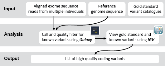
This is an example interpretation of the results from this recipe. In our Galaxy workflow we first used FreeBayes to compare our short-read exome sequencing alignments to a reference sequence in order to determine likely genetic variants in our sample cohort. Next we used VCFfilter to filter these results for high quality variants based on various metrics (e.g., read depth, quality score). We also used VCFintersect to further narrow our results down to those variants with equivalent alleles in the HapMap catalog. Finally, we turned to IGV to view our filtered variants alongside a set of known pathogenic variants identified in the dbSNP database. Specifically, we would like to see if any of our identified variants may be associated with an increased risk for disease.

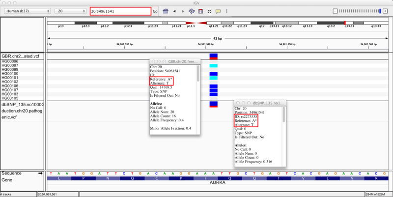
We zoom in on a specific variant located in the q13.31 cytoband of chromosome 20 by typing the coordinates 20:54961541 into the regions navigation bar and hitting enter. Both our results track (upper) and dbSNP track (lower) display a variant at this site, as indicated by the blue and red bar (the proportion of red in the bar corresponds to the allele frequency of the variant). The group of 10 tracks display the genotypes of the 10 individuals whose sequences we used in this recipe. Specifically, 4 individuals are heterozygous for the variant (blue), 2 individuals are homozygous (cyan), and the remaining 4 individuals are homozygous (grey) for the reference allele.

Clicking on the variants in either track brings up info-boxes that display various statistics for the variant. By comparing to the dbSNP track, we notice that our variant analysis has identified an A/T SNP that corresponds to the pathogenic variant, rs2273535, in the AURKA gene. Moreover, our set of 10 samples carried the minor allele with a frequency of 0.4, which corresponds closely to the allele frequency of 0.316 reported in the dbSNP annotations. Given this correspondence, we reason that we have identified the pathogenic SNP rs2273535 in our sample set of 10 British individuals. If we search for SNP id rs2273535 in ClinVar (link), we see that it has been identified as a risk factor for colon cancer. However, note that due to our small sample size these variant discoveries may not be generalizable to the whole population; this is only a simple representation of possible results.


Posted by mvila on December 18, 2017 12:09

Hi, I've been trying to follow this recipe, but could not launch the data to Galaxy. Please check, whether there is any problem with that. Thanks, Marta

Posted by ted on December 18, 2017 17:12

Marta, it looks like the GenomeSpace importer in Galaxy has been updated and in the new version it does not allow multiple files to be imported at once. I am contacting the developer and will try to get this corrected. I will contact you via email to follow up. Thanks for letting us know, Ted

Submit a Comment

History