Gp to cytoscape3

Find subnetworks of differentially expressed genes and identify associated biological functions

Added by GenomeSpaceTeam on 2015.03.16 Official logo
Last updated on over 3 years ago.


Summary

What subnetworks of differentially expressed genes are enriched in my samples? What biological functions are they related to?

This recipe provides a method for identifying differentially expressed genes between two phenotypes, such as tumor and normal, to find subnetworks of interacting proteins and determine their functional annotations. An example use of this recipe is a case where an investigator may want to compare two phenotypes to determine which gene networks are similar between phenotypes, and to determine how functional annotation changes between phenotypes.


In particular, this recipe makes use of several GenePattern modules to identify differentially regulated genes, then uses several Cytoscape plugins to identify potential interactions between gene products, and to visualize the resulting network.

Why differential expression analysis? We assume that most genes are not expressed all the time, but rather are expressed in specific tissues, stages of development, or under certain conditions. Genes which are expressed in one condition, such as cancer tissue, are said to be differentially expressed when compared to normal conditions. To identify which genes change in response to specific conditions (e.g. cancer), we must filter or process the dataset to remove genes which are not informative.

Why protein interaction network analysis? Gene expression analysis results in a list of differentially expressed genes, but it does not explain whether these genes are connected biologically in a pathway or network. To better understanding the underlying biology that drives changes in gene expression analysis, we can perform network analysis to determine whether gene products (e.g. proteins) are reported to interact. To identify potential networks or pathways, we search for highly interconnected subnetworks within a large interaction network.

Inputs

To complete this recipe, we will need a gene expression dataset describing two conditions or phenotypes, such as cancer tissue vs. normal tissue. In this example, we will use gene expression data from a study in which committed granulocyte macrophage progenitor cells (normal phenotype) were transformed into leukemia stem cells (leukemic phenotype) by introduction of the MLL-AF9 protein. This example data is derived from mouse (Mus musculus) cell lines. We will need the following datasets, which can be downloaded from the following GenomeSpace Public folder:

Public > RecipeData > ExpressionData: Normal_Leu.gct: This file contains gene expression data of two phenotypes: normal and leukemic. The file is available in GenePattern's GCT format.

Public > RecipeData > ExpressionData: Normal_Leu.cls: This file contains class assignments (normal or leukemic) for all the samples in the GCT file, as identified by the GenePattern CLS format.

Outputs

The visual representation of a subnetwork of differentially expressed genes.

Recipe steps

  • GenePattern
    1. Loading data
    2. Filtering genes by expression value
    3. Identifying differentially expressed genes
    4. Selecting the top genes
    5. Save the files to GenomeSpace
  • Cytoscape 3
    1. Loading data into Cytoscape
    2. Identifying interacting proteins
    3. Finding differentially expressed subnetworks
    4. Exploring the subnetworks

NOTE: If you have not yet associated your GenomeSpace account with your GenePattern account, you will be asked to do so. If you do not yet have a GenePattern account, you can automatically generate a new account that will be associated with your GenomeSpace account.

  1. Open GenePattern from GenomeSpace, navigate to the GenomeSpace tab, then navigate to your personal directory.

1. Click on the file (e.g., Normal_Leu.gct) in GenomeSpace, then use the GenePattern context menu and click Launch on File.

OR

2. Click on the file (e.g., Normal_Leu.gct) in GenomeSpace, then drag it to the GenePattern icon to launch.


  1. Change to the Modules tab, and search for "PreprocessDataset".
  2. Once the module is loaded, change the following parameters:
    1. input filename: load the GCT file, e.g., Normal_Leu.gct. To do this, navigate to the GenomeSpace tab, and navigating to the folder containing the GCT file: Public > RecipeData > ExpressionData. Load the file into the input filename parameter by clicking and dragging the file to the input filename input box.
  3. Click Run to run PreprocessDataset. This will generate a processed GCT file.

  1. Change to the Modules tab, and search for "ComparativeMarkerSelection".
  2. Once the module is loaded, change the following parameters:
    1. input file: load the processed GCT file, e.g., Normal_Leu.preprocessed.gct. To do this, navigate to the Jobs tab, and find the preprocessed GCT file from the previous job. Click and drag the file to the input file input box.
    2. cls file: load the CLS file, e.g., Normal_Leu.cls. To do this, navigate to the GenomeSpace tab, and navigating to the folder containing the CLS file: Public > RecipeData > ExpressionData. Click on the file and choose Send to cls file, or by dragging the file to the cls file input box.
  3. Click Run to submit your job. This will generate an ODF file.

  1. Change to the Modules tab, and search for "ExtractComparativeMarkerResults".
  2. Once the module is loaded, change the following parameters:
    1. comparative marker selection filename: load the ODF file from the previous job, e.g., Normal_Leu.preprocessed.comp.marker.odf. To do this, navigate to the Jobs tab, and find the processed ODF file from the previous job. Click and drag the file to the comparative marker selection filename input box.
    2. dataset filename: load the processed GCT file, e.g., Normal_Leu.preprocessed.gct. To do this, navigate to the Jobs tab, and find the preprocessed GCT file from a previous job. Click and drag the file to the dataset filename input box.
    3. statistic: Rank
    4. max: 50
  3. Click Run to submit your job. This will generate two filtered files, a filtered GCT file, and a filtered TXT file.

  1. Change to the Modules tab, and search for "SelectFileMatrix".
  2. Once the module is loaded, change the following parameters:
    1. input file: load the filtered GCT file, e.g., Normal_Leu.preprocessed.comp.marker.filt.gct. To do this, navigate to the Jobs tab, and find the processed GCT file from the previous job. Click and drag the file to the input file input box.
    2. output file base name: set the output file base name parameter to a new output file name, e.g., Normal_Leu.genes.
    3. start row: 3
    4. end row: 53
    5. start column: 2
    6. end column: 2
      NOTE: to keep more information from this gene list, e.g. the values in the remaining columns, set the start column and end column parameters to be blank. This will select all the columns in the file.
  3. Click Run to submit your job. This will generate a new TXT file which contains only the gene names (column 2), with the first row as a header, e.g., Normals_Leu.genes.txt.


Save the Normals_Leu.genes.txt file to GenomeSpace using one of the following methods.

  1. From the job processing view, click the context menu (blue arrow) next to the dataset (e.g., Normals_Leu.genes.txt), then choose Save to GenomeSpace. Save the file to your folder.
  2. From the Modules and Pipeline start page, navigate to Jobs. Click on the file, then choose Send to GenomeSpace. Save the file to your folder.
  3. OPTIONAL: close GenePattern.
  1. Launch Cytoscape from GenomeSpace by clicking on the Cytoscape icon in the tool menu, prompting the download of a cytoscape.jnlp file. Double-click the file to launch Cytoscape.
  2. Once Cytoscape has launched, it will prompt a start menu. Under the Start New Session label, choose With Empty Network.

  3. Once the Cytoscape 3 software has loaded, it will prompt the user to name their network. Feel free to change the network name, or leave the parameters as default. Click OK.

  4. To load files, navigate to the GenomeSpace import menu: File > Import > Network > GenomeSpace.

  5. Navigate to the file which contains the gene names, e.g., Normals_Leu.genes.txt. Choose Select to load the file. This will load a new menu for importing a network from a table.
  6. In the Import Network From Table box, click the arrow to expand the menu. If no arrow appears, continue to step 8.

  7. Under the Meaning: box, choose the green circle icon that designates "source interaction".
  8. Click OK to import the file.
  9. Cytoscape will prompt a warning that only nodes are being imported, and that no interactions/edges will be generated. Click Yes to confirm that the network should be imported.

    You should see many nodes (gene names), but no interaction edges.
  10. Under the Table Panel, select all the node ID names by clicking on the top/first node name (e.g. "Trf"), then choosing shift and scrolling downward. Then use ctrl+c (Windows) or ctrl+click (Mac) to copy the list of names.
  1. To install GeneMANIA, navigate to Apps > AppManager.

  2. Install GeneMania using the following method:
    1. Under Install Apps, search for "GeneMANIA".
    2. Click on the tool name.
    3. Click Install. This may take several minutes.
    4. Once the app has installed, click Close.
  3. If you've already installed GeneMania, navigate to: Apps > GeneMANIA > Search.
    NOTE: if you have never run GeneMANIA before, you will be prompted to install a database. Use the following steps:
    1. Click Install Data....
    2. Under the Download tab, choose Mus musculus Mouse.
      NOTE: You may use your own database files; however, the species should match that of your expression data; i.e., if you are using H. sapiens data, make sure the database is also from H. sapiens.
    3. Click Install. This may take several minutes.
    4. Once the database is installed, click Close.
  4. Once GeneMANIA is loaded, change the following parameters:
    1. Organism: M. musculus (mouse). If you are using your own database, make sure to select the appropriate species.
    2. Genes of Interest: Click the empty box, then ctrl+v (Windows) or ctrl+click (Mac) to load your gene list into GeneMANIA.
      NOTE: A dialog box may appear, telling you that some genes were not found in the GeneMANIA database; you can click OK.
  5. Click Start to begin identifying connections between genes. This may take several minutes. Once the job is complete, close the GeneMania pop-up.
  1. To install MCODE, navigate to Apps > AppManager.
  2. Install MCODE using the following method:
    1. Under Install Apps, search for "MCODE".
    2. Click on the tool name.
    3. Click Install. This may take several minutes.
    4. Once the app has installed, click Close.
  3. In Cytoscape, navigate to the MCODE plugin: Apps > MCODE > Open MCODE.
  4. Once MCODE is loaded, it will create a new tab in the Control Panel. To run MCODE, change the following parameters:
    1. Find Cluster(s): in Whole Network
    2. Click the arrow next to Advanced Options
    3. Cluster Finding: Check the Haircut parameter.
  5. Click Analyze the Current Network to identify subnetworks in your network. The results from this search will appear in the Results Panel on the upper right.

  • To highlight the proteins in a cluster, select the cluster in the Results Panel. This will also list the proteins in the Table Panel.
  • Cytoscape provides many options for displaying a network. For example:
    • A spring-embedded layout finds an optimal way to display nodes and edges by simulating nodes as objects and edges as springs connecting objects together. Cytoscape provides several variations on a spring-embedded layout. To create a spring-embedded layout, navigate through the following menu:
      Layout > Edge Weighted Spring Embedded Layout
    • A circular layout arranges nodes in a circle. Layouts can use information about a node, such as the node's degree, to determine the order of nodes within the circle. To create a circular layout, navigate through the following menu:
      Layout > Circular Layout
  • To control the density of the network (how far nodes are from one another), you can use the Scale function. Select Layout > Scale, then use the sliding scale bar to increase or decrease network density.
  • To change the visual style of the network, e.g., by coloring nodes or adding arrows to edges, navigate to the Style tab in the Control Panel. You can choose preset styles using a drop-down menu. You can create your own styles by clicking on the Defaults pane, then adjusting the parameters.
    For example, to adjust edge color first choose the Edge tab in the bottom part of the pane. Then click on EDGE_COLOR, choose a new color, and click OK. Some variables take numeric inputs, such as EDGE_LINE_WIDTH.

Results Interpretation

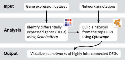
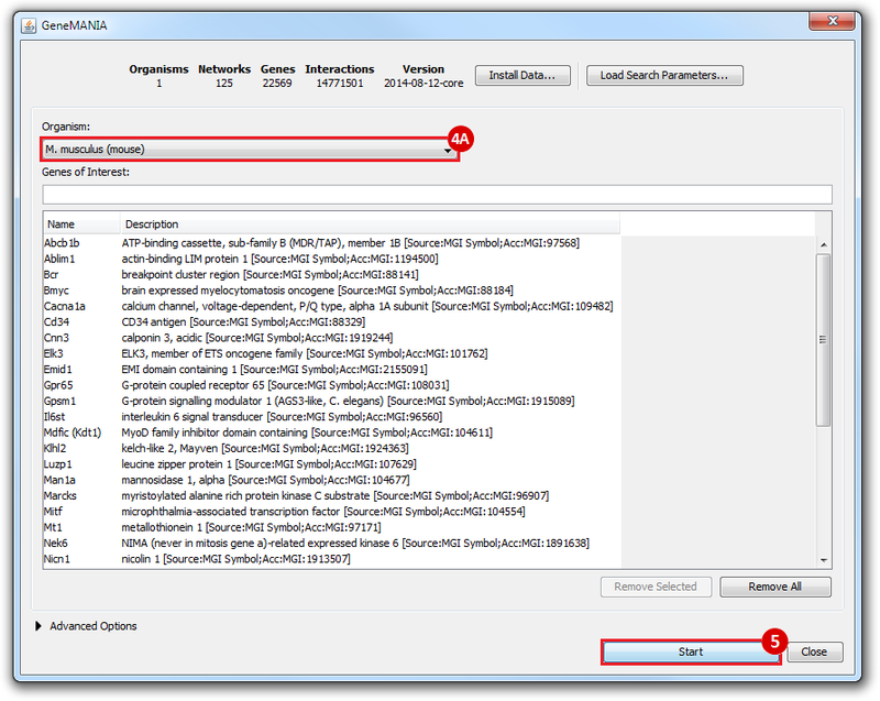
This is an example interpretation of the results from this recipe. First, we identified the top 50 genes which differentiated between two phenotypes, leukemic and normal. We then used the GeneMANIA tool in Cytoscape to identify connections between these genes, although some genes were not annotated and therefore only a subset were actually analyzed. We included all possible sources of interaction, i.e. we are equally interested in connections between genes that arise from co-expression, as we are in connections arising from physical interactions.
After running GeneMANIA we created a network which connected our subset of genes. We can see from the GeneMANIA results that, e.g. 3 genes (out of 45) have the Gene Ontology (GO) annotation 'zinc ion homeostasis', which has a total of 16 genes associated with it. The significance of this enrichment is reported as a q-value, calculated from a FDR corrected hypergeometric test for enrichment. The q-value is analogous to a p-value, and therefore a lower q-value is considered more significant.

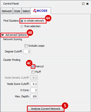
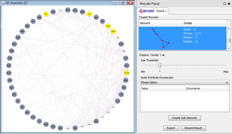
Once we learn about the functional enrichment associated with the genes in our network, we are interested in determining whether we can find subnetworks, i.e. areas of the network which have motifs. We use MCODE to identify subnetworks. For example, MCODE identifies a small subnetwork of 5 nodes and 6 edges. When we click on this subnetwork in the MCODE panel, it will highlight the nodes in the network.

We can separate this set of genes into a subnetwork by clicking the Create sub-network button in MCODE. This generates a new view containing the subnetwork, arranged according to the MCODE subnetwork view. Looking at this subnetwork of genes, we can examine their annotation and see that 3 of these genes are associated with zinc ion binding.

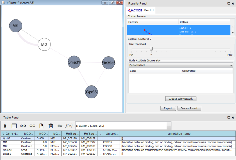
These results suggest that there is a collection of zinc ion binding genes in our set of 50 genes which differentiated between leukemic and normal phenotypes. However, the results in this example are not necessarily significant and are only a simple representation of possible results.


Submit a Comment

History