Gp galaxy

Eliminate batch effects in RNA-seq data

Added by GenomeSpaceTeam on 2016.03.08 Official logo
Last updated on over 3 years ago.


Summary

Does my RNA-Seq data contain noticeable batch effects? Can I remove any batch effects I find?

This recipe provides one method to assess RNA-seq count data for potential batch effects. Identified batch effects are removed using the ComBat algorithm (Johnson, Rabinovic, and Li). An example use case of this recipe is when an investigator wants to correct data and account for confounding variables generated by effects such as using different reagents or processing samples at different times.


This recipe uses count data and sample annotations derived from two separate RNA-seq experiments and relies upon Principal Component Analysis (PCA) as a primary means of evaluating the dataset for batch effects. In particular, this recipe utilizes a number of GenePattern modules to filter and preprocess the RNA-seq count data and to normalize the dataset using the ComBat algorithm. We then use Galaxy to view the influence of batch effects in our pre- and post-normalization datasets.

Why consider batch effects (a.k.a. confounders)? A "batch" or "confounding" variable can be generally defined as an extraneous variable that may correlate or anti-correlate with our variables of interest. Failing to account for confounding variables or batch effects can lead us to draw spurious conclusions from our data. For example:

Albert is comparing the hardiness of two different E. coli strains, X and Y, by measuring their production of various stress proteins under a mild bactericide. However, Albert's bactericide stock is running low and he ends up using two different stocks of the same bactericide over the course of this experiment. Here, bactericide stock is a confounding or batch variable. Perhaps one bactericide stock is more potent than the other. Albert will need to be careful in how he analyzes his data. He must somehow ensure that differences in stress protein abundances between his X and Y strains are driven by the biological differences of these two strains rather than differences in the bactericide stocks.

Efforts can be undertaken to minimize batch effects by ensuring proper experimental design, e.g., simplifying protocols to eliminate potential confounders. If batches are unavoidable, it is also important to randomize samples across these batches such that differences between batches can be attributed to batch effects rather than biological differences. But despite these efforts, unforeseen batch effects may still be present in any experiment. Thus, we should be aware of the degree to which these unwanted factors influence our results and be prepared to use various statistical methods to remove these unwanted factors if needed.

How do we identify batch effects? There are a variety of methods for identifying batch effects. Sometimes, potential batches can be identified at the outset of a project based on its experimental design. For example, if samples must be processed in separate groups due to the limiting capacity of a sequencer, then these processing groups are likely to introduce batch effects. If batches can be pre-identified, then the scientist can include identical control samples in each batch. Any variation in measurements from these control samples can then be attributed to and used to quantify a batch effect.

Another common method is to visualize data using a PCA projection. PCA uses a linear transformation to transform a dataset into a space of linearly uncorrelated, orthogonal "principal components". More simply, PCA is a way of visualizing data such that underlying structures are revealed. We encourage users to learn more about PCA (Ma and Dai's 2011 article in Briefings in Bioinformatics is a good starting point). By re-projecting with PCA, we can identify those variables, including batch variables, that are contributing to large variances in the dataset.

Inputs

To complete this recipe, we will need a gene expression dataset of RNA-seq transcript counts describing multiple conditions or phenotypes that may be confounded due to batch effects. In this example, we will use a dataset combining gene expression measurements from two mouse (Mus musculus) behavior studies. In the first study (GEO: GSE63412), Peixoto et al. subjected animals to contextual fear conditioning (FC) and compared them to unconditioned controls. In the second study (GEO: GSE44229), Vogel-Ciernia et al. subjected animals to object location memory (OLM) training and compared them to unconditioned homecage controls. In both studies, samples destined for expression profiling were collected from hippocampal tissue. In this particular recipe, we have pre-combined the two studies into a single RNA-seq count dataset, which we will use. The known batch effect in this dataset is thus the two different labs generating the RNA-seq data.

NOTE: Since this is an example dataset for the purposes of demonstrating batch effects and their removal, we have chosen to construct a dataset that can dramatically show the effects of confounders. We therefore chose to combine two similar datasets from different labs, knowing that lab would be a strong confounding variable. When combining datasets, great care should be taken to ensure that the samples and data-generation procedures are truly comparable. This particular combination of two mouse behavioral conditioning datasets may not meet these requirements. When working with your own datasets, you may find that batch effects are not as clearly defined or that the data's underlying structure cannot be easily attributed to known confounding variables. Your confounding variables will probably be more subtle than the differing labs of our example (e.g., differing instrumentation, variable reagents, time of sample collection).

This recipe also requires a relatively detailed sample annotation file indicating each sample's name, behavioral condition, and the lab from which it was derived. We have already compiled these sample annotations as both a sample information file and a CLS class file. We will need the following datasets, which can be downloaded from the following GenomeSpace Public folder:

Public  >  RecipeData  >  ExpressionData  >  GSE63412_GSE44229.gct: This is an expression matrix containing hippocampal RNA-seq count data from mice that were subjected to a variety of behavioral training protocols. Importantly, we are interested in performing a combined analysis using data from two different laboratories; the expression matrix likely has underlying batch effects that should be removed prior to any downstream analysis. The read count data was obtained and compiled from the Gene Expression Omnibus. The file is available in GenePattern's GCT format.

Public  >  RecipeData  >  ExpressionData  >  GSE63412_GSE44229.sample.info.txt: This is a table of annotations for all the samples in the GCT file. The "Batch" column indicates the sample's originating laboratory, which we treat as our confounding "batch" variable. The "Covariate_1" column lists the actual behavioral training that each animal received (control, fear conditioning, object location memory training).

Public  >  RecipeData  >  ExpressionData  >  GSE63412_GSE44229.cls: This file contains class assignments (control, fear conditioning, object location memory training) for all the samples in the GCT file. The file is available in GenePattern's CLS format.

Outputs

This recipe generates a gene expression dataset in log counts-per-million from RNA-seq count data. This expression dataset has been filtered for lowly expressed reads and adjusted for an identified batch effect using the ComBat tool. This recipe also generates Principal Component Analysis plots of the expression dataset both prior to and after adjustment for batch effect.

Recipe steps

  • GenePattern
    1. Filter and convert read counts to logCPM
    2. Remove batch effects using ComBat and save output to GenomeSpace
    3. Extract high-variance genes from pre- and post-ComBat expression datasets
  • Galaxy
    1. Loading data into Galaxy
    2. Prepare expression datasets for PCA
    3. Perform PCA on pre- and post-ComBat expression datasets
    4. Visualize the expression datasets in the space of their first two principal components

  1. Under the Modules tab, search for "PreprocessReadCounts".
  2. Once the module is loaded, change the following:
    1. input file: Load the GCT file. To do this, open the GenomeSpace tab, and navigate to the folder containing the GCT file (e.g. Public  >  RecipeData  >  ExpressionData  >  GSE63412_GSE44229.gct). Load the file into the input file parameter by clicking and dragging the file to the input file input box.
    2. cls file: Load the CLS file. To do this, open the GenomeSpace tab, and navigate to the folder containing the CLS file (e.g. Public  >  RecipeData  >  ExpressionData  >  GSE63412_GSE44229.cls). Load the file into the cls file parameter by clicking and dragging the file to the cls file input box.
    3. output file: <input.file_basename>.logcpm.gct
  3. Click Run to submit your job. This will generate a GCT file of the expression data in logCPM.

  1. Under the Modules tab, search for "ComBat".
  2. Once the module is loaded, change the following parameters:
    1. input file: load the filtered, logCPM GCT file, e.g., GSE63412_GSE44229.logcpm.gct. To do this, navigate to the Jobs tab, and find the processed GCT file from the previous job. Click and drag the file to the input file input box.
    2. sample info file: Load the sample info file. To do this, navigate to the GenomeSpace tab, and navigate to the folder containing the file (e.g. Public  >  RecipeData  >  ExpressionData  >  GSE63412_GSE44229.sample.info.txt). Load the file into the sample info file parameter by clicking and dragging the file to the sample info file input box.
    3. prior method: Ensure that this parameter is set to "parametric".
  3. Click Run to submit your job. This will generate a GCT file of the expression data that has been normalized for batch effects as well as a JPEG file of prior probability distribution plots.


Save the GSE63412_GSE44229.logcpm.combat.gct file (and optionally the GSE63412_GSE44229.logcpm.combat.plot.jpeg file) to GenomeSpace for later reference using one of the following methods:

  1. From the job processing view, click the context menu (blue arrow) next to the dataset (e.g., GSE63412_GSE44229.logcpm.combat.gct), then choose Save to GenomeSpace. Save the file to your folder.
  2. From the Modules and Pipeline start page, navigate to Jobs. Click on the file, then choose Save to GenomeSpace. Save the file to your folder.
  1. Under the Modules tab, search for "PreprocessDataset".
  2. Once the module is loaded, change the following parameters:
    1. input filename: load the ComBat-processed GCT file, e.g., GSE63412_GSE44229.logcpm.combat.gct. To do this, navigate to the Jobs tab, and find the batch effect normalized GCT file from the previous job. Click and drag the file to the input file input box.
    2. floor: -100
    3. ceiling: 100
    4. min fold change: 0
    5. min delta: 1.5
    6. output file: <input.filename_basename>.hidelta


      Note: By selecting a minimum delta threshold, we restrict the expression datasets to a list of ~900 highly variant genes. Here, we used delta thresholding to perform this restriction, with limits specifically chosen to give ~900 genes from both datasets. Alternative methods include explicitly ranking genes by variance and selecting the n most highly variant genes. Since PCA transforms the data to a system of coordinates that capture the variance in the data, it is typical to limit a dataset to a smaller number of highly variant features prior to applying PCA. This feature reduction simplifies the downstream process of calculating principal components while ensuring that the transformation will remain faithful to the structure of the overall dataset.

  3. Click Run to submit your job. This will generate a GCT file of the expression data that has been filtered for genes with high-delta values across the experiment.
  4. Rerun PreprocessDataset on the pre-ComBat GCT file. To do this, reload the previous job by navigating to the Jobs tab, clicking on the relevant PreprocessDataset job title, and selecting Reload Job.  Then make the following parameter changes:
    1. input filename: load the pre-ComBat GCT file, e.g., GSE63412_GSE44229.logcpm.gct. To do this, navigate to the Jobs tab, and find the logCPM GCT file from a previous job. Click and drag the file to the input file input box.
    2. min delta: 2.5
    3. Click Run to submit your job.
  5. Save the GSE63412_GSE44229.logcpm.hidelta.gct and GSE63412_GSE44229.logcpm.combat.hidelta.gct files to GenomeSpace using one of the following methods:
    1. From the job processing view, click the context menu (blue arrow) next to the dataset (e.g., GSE63412_GSE44229.logcpm.hidelta.gct), then choose Save to GenomeSpace. Save the file to your folder.
    2. From the Modules and Pipeline start page, navigate to Jobs. Click on the file, then choose Save to GenomeSpace. Save the file to your folder.
  6. OPTIONAL: close GenePattern.

NOTE: If you have not yet associated your GenomeSpace account with your Galaxy account, you will be asked to do so. If you do not yet have a Galaxy account, you can automatically generate a new account that will be associated with your GenomeSpace account.

  1. Click on the Galaxy icon to launch the tool.
  2. Navigate to the following menu: Get Data > GenomeSpace import
  3. Select the GSE63412_GSE44229.logcpm.hidelta.gct, GSE63412_GSE44229.logcpm.combat.hidelta.gct, and GSE63412_GSE44229.sample.info.txt files; ensure that the Send As fields are set as follows:
    1. GSE63412_GSE44229.logcpm.hidelta.gct: genomicatab
    2. GSE63412_GSE44229.logcpm.combat.hidelta.gct: genomicatab
    3. GSE63412_GSE44229.sample.info.txt: txt
  4. Click Send to Galaxy.
  5. Once the files have been loaded, change the attributes for each file, by clicking the pencil () icon. Switch to the Datatype tab and changing the following parameters:
    1. New type: tabular
    2. Click Save. Ignore any warnings which may pop up.
  1. Within Galaxy, click on the Workflow tab to open the main Workflow page.
  2. Click the Upload or import workflow button in the upper right corner to begin importing a workflow.
  3. Copy the URL below and paste it in the Galaxy workflow URL: field. Click Import to import the workflow into your Galaxy environment.
  4. Click on the workflow drop-down menu (e.g., Identifying batch effects – PCA Preprocessor (imported from uploaded file)), then choose Run.
  5. Load the files into the correct fields. The input fields should have annotations indicating which file should be loaded:
    1. Step 1: Input Dataset: GSE63412_GSE44229.logcpm.hidelta.tab
    2. Step 2: Input Dataset: GSE63412_GSE44229.logcpm.combat.hidelta.tab
  6. Click Run workflow.

  1. Navigate to the following menu: Multivariate Analysis > Principal Component Analysis
  2. Once the tool is loaded, change the following parameters:
    1. Select data: Transpose: Preprocessed Pre-ComBat expr data
    2. Select columns containing input variables: Check the box next to Select/Unselect all (Note: This step may take some time as we are specifying hundreds of columns as our input variables; after selecting the box, wait for the variable names to populate the form before proceeding.)
    3. Method: Singular Value Decomposition (prcomp)
    4. Centering and Scaling: Center only
  3. Click Execute.
  4. Repeat steps 1 through 3 on the post-ComBat GCT file (Transpose: Preprocessed Post-ComBat expr data).

  1. Within Galaxy, click on the Workflow tab to open the main Workflow page.
  2. Click the Upload or import workflow button in the upper right corner to begin importing a workflow.
  3. Copy the URL below and paste it in the Galaxy workflow URL: field. Click Import to import the workflow into your Galaxy environment.
  4. Click on the workflow drop-down menu (e.g., Identifying batch effects – PCA Viewer (imported from uploaded file)), then choose Run.
  5. Load the files into the correct fields. The input fields should have annotations indicating which file should be loaded:
    1. Step 1: Input Dataset: GSE63412_GSE44229.sample.info.txt
    2. Step 2: Input Dataset: PCA on the Pre-ComBat expr data (Note: the Principal Component Analysis tool generates two output files; we require the tabular output for the workflow, not the pdf output)
    3. Step 3: Input Dataset: PCA on the Post-ComBat expr data (Note: the Principal Component Analysis tool generates two output files; we require the tabular output for the workflow, not the pdf output)
  6. Click Run workflow.

  1. Once the workflow has completed, click on the Paste: Viz of Pre-ComBat PCA output file to access more options; click the graph() icon and select Charts from the dropdown menu to begin plotting the results.
    1. Under the Start tab, select Scatter plot (NVD3)
    2. Under the Customize tab, set the parameters:
      1. X axis > Axis label: PC 1
      2. Y axis > Axis label: PC 2
    3. Click the Select Data tab; for 1: Data Series, set the parameters:
      1. Provide a label: LabA
      2. Data point labels: Column: 9
      3. Values for x-axis: Column: 11
      4. Values for y-axis: Column: 12
    4. Click the Insert Data tab; for 2: Data Series, set the parameters:
      1. Provide a label: LabB
      2. Data point labels: Column: 3
      3. Values for x-axis: Column: 5
      4. Values for y-axis: Column: 6
  2. Click the Visualize button in the upper right-hand corner. (Optional: Save a screenshot of the visualization)
  3. Repeat steps 7 and 8 on the Paste: Viz of Post-ComBat PCA output file.

Results Interpretation

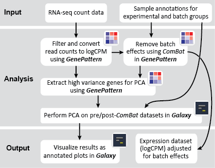
There are two primary goals of this recipe: (1) identify potential batch effects in our dataset and (2) adjust our data for any identified batch effects. This recipe generates a number of plots to help us evaluate our data along these aims:

Figure 1. Viz_of_PreComBat_PCA.pdf Figure 2. GSE63412_GSE44229.logcpm.combat.plot.jpeg Figure 3. Viz_of_PostComBat_PCA.pdf
PCA of expression data prior to applying ComBat, colored by originating lab. Prior plots of parametric ComBat algorithm. Parametric estimates of batch effect are in red; kernel density estimate of batch effect are in black. PCA of expression data after applying ComBat, colored by originating lab./td>
This figure was obtained from Step 7: Visualize the expression datasets in the space of their first two principal components. This figure was obtained from Step 2: Remove batch effects using ComBat and save output to GenomeSpace. This figure was obtained from Step 7: Visualize the expression datasets in the space of their first two principal components.


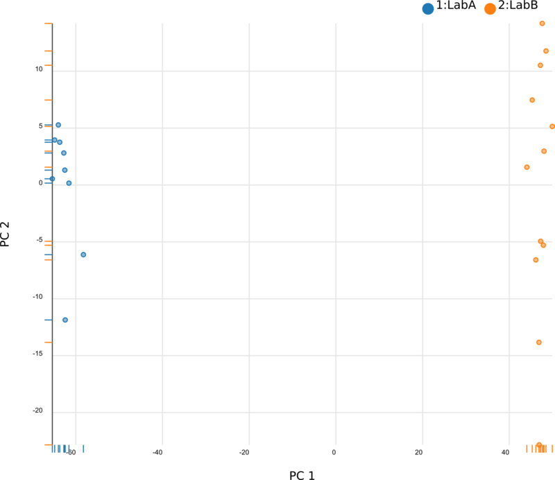
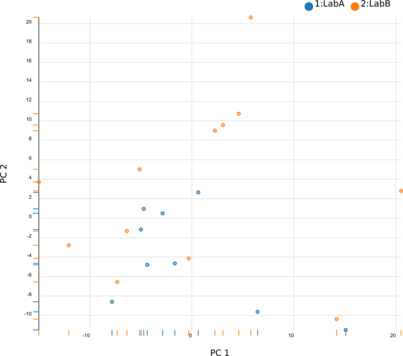
We began by using Principal Component Analysis (PCA) to view the underlying structure of our raw expression data prior to applying ComBat. To do this, we projected our data in the space of the first two principal components, PC1 and PC2, with each point representing a different sample from the experiment (Fig. 1). The PCs identified by PCA transformation are ordered such that the first principal component, PC1, captures the largest possible variance in the dataset, and each following PC captures the highest variance possible while being orthogonal to the previous PCs. If we view our pre-ComBat data, we clearly see that the samples cluster according to the lab (Lab A or Lab B) that they came from. Since these clusters are located at disparate ends of PC1, it appears that the originating lab introduces much (if not most) of the variance in our dataset. We conclude that the lab in which the samples were processed is a batch effect.

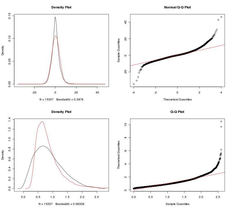
To adjust our dataset for the identified batch covariate, Lab, we used ComBat. ComBat requires that we specify this batch covariate as well as covariates of interest; in this case, we were interested in a single covariate, treatment (control, fear conditioning, object location memory). The parametric ComBat method that we used computes a prior probability distribution for the adjustment. To evaluate this prior distribution, we view the prior plots that the ComBat algorithm outputs (Fig. 2). In this case, the parametric estimate (red) overlaps the "true" distribution (black, kernel density estimate) pretty well, so we can feel reasonably confident in our ComBat adjustment. In the case of poor estimates, we would resort to the non-parametric setting for the algorithm. For more information, see GenePattern's documentation on ComBat.

After applying ComBat to our expression dataset, we again apply PCA and project the transformed data into the space of the first two PCs (Fig. 3). Post-ComBat, we see that the samples from our two lab groups are more overlapping, indicating that the batch effect has been mitigated.

At this point, the investigator can proceed in number of directions. The post-ComBat PCA projection can be explored to see how our covariates of interest cluster. Moreover, the ComBat-adjusted dataset (GSE63412_GSE44229.logcpm.combat.gct) can be used in downstream expression analysis (e.g., differential expression analysis).

References

  1. Johnson WE, Rabinovic A, and Li C. Adjusting batch effects in microarray expression data using Empirical Bayes methods. Biostatistics. 2007;8(1):118-127. PMID: 16632515
  2. Ma S and Dai Y. Principal component analysis based methods in bioinformatics studies. Brief Bioinform. 2011 Nov;12(6):714-22. PMID: 21242203
  3. Peixoto L, Risso D, Poplawski SG, Wimmer ME et al. How data analysis affects power, reproducibility and biological insight of RNA-seq studies in complex datasets. Nucleic Acids Res. 2015 Sep 18;43(16):7664-74. PMID: 26202970
  4. Vogel-Ciernia A, Matheos DP, Barrett RM, Kramár EA et al. The neuron-specific chromatin regulatory subunit BAF53b is necessary for synaptic plasticity and memory. Nat Neurosci. 2013 May;16(5):552-61. PMID: 23525042

Submit a Comment

History