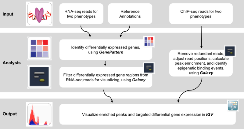
This is an example interpretation of the results from this recipe. We used MACS2 in Galaxy to identify differentially read-enriched regions in mouse embryonic stems cells possessing the Prep1 transcription factor binding to those that did not. The specific configuration of MACS2 we use calls narrow peaks, in other words enriched regions highly associated with transcription factor binding sites, as opposed to broad peaks, which are more highly associated with histone modifications. Additionally, we have portrayed the landscape of binding events in both samples (Knockout and Wild-type). In conjunction, we wanted to identify how this transcription factor binding regulated nearby genes. Using the GenePattern module, Cufflinks, were were able to identify genes that were significantly (p<0.05) differentially expressed between samples. Below is an example of how this data can be visualized in IGV.
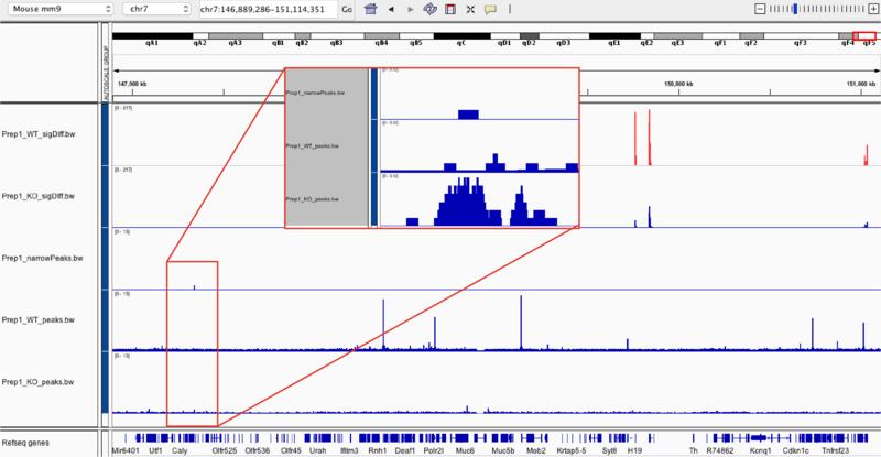
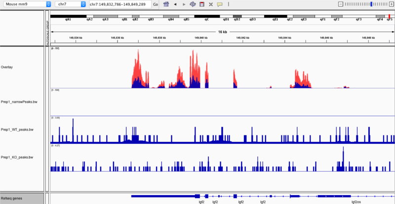
Below highlights the narrow peak identified in comparing transcription factor occupancies between embryonic stem cells with the knockout (Prep1_KO_peaks.bw) and those with Prep1 (Prep1_WT_peaks.bw) binding in the chr7:149,889,286-151114351 region.
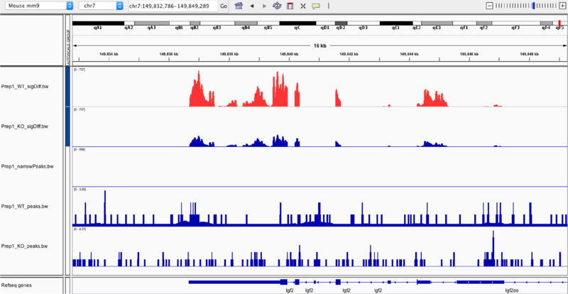
In the top two frames are the gene expression profiles of the wild-type (first) and the knock-out (second) samples. By zooming in to the chr7:149,832,786-149,849,289 region, we are able to compare the gene expression profiles, especially when we overlay the two samples (seen far below). In overlaying, we can identify whether the type of regulation (up or down) that occurs in relation to the Prep1 transcription factor binding.

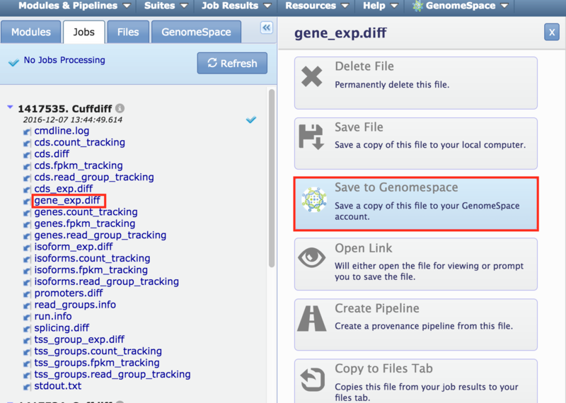
 GenomeSpace.org


 , to import the workflow into your Galaxy environment.
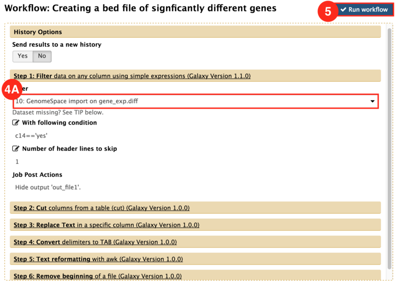
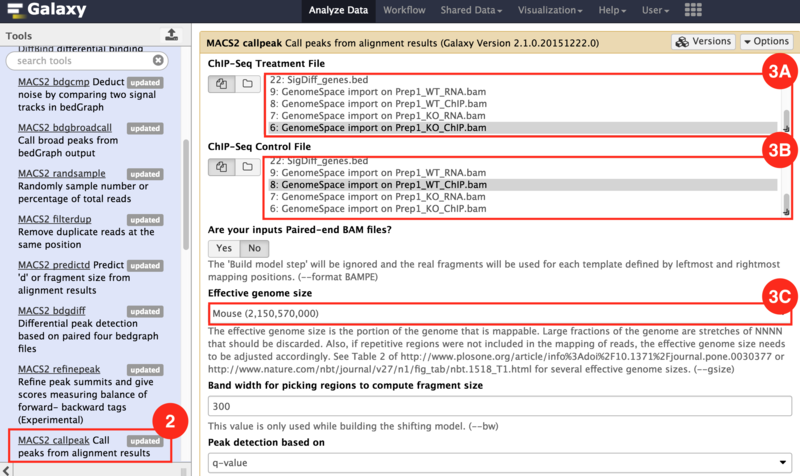
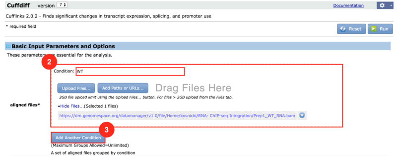
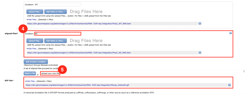
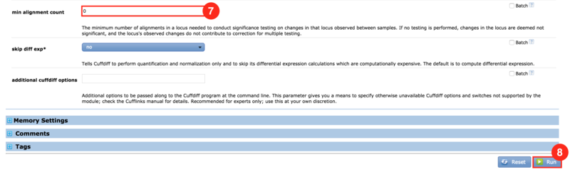
 ) to input both the WT and KO aligned reads.
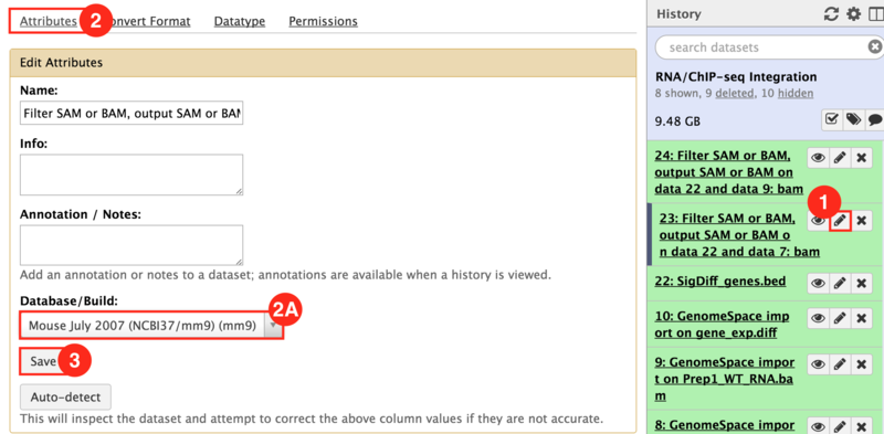
 ) icon.