Content ucsc gp igv

Find differentially expressed genes in RNA-seq data

Added by GenomeSpaceTeam on 2015.04.21 Official logo
Last updated on over 3 years ago.


Summary

Which genes are differentially expressed between my two phenotypes, based on my RNA-seq data?

This recipe provides one method to identify differentially expressed genes in RNA-seq read data. An example use of this recipe is a case where an investigator may want to compare two phenotypes, such as two types of cancer, to determine which genes are up- or down-regulated differently between these phenotypes.


In particular, this recipe uses the UCSC Table Browser to retrieve a reference genome to align RNA-seq reads against. We also used several modules in GenePattern to align the reads against the reference genome, and to identify differentially expressed genes when comparing two conditions. Finally, we use IGV to visualize the differentially expressed genes.

Why differential expression analysis? We assume that most genes are not expressed all the time, but rather are expressed in specific tissues, stages of development, or under certain conditions. Genes which are expressed in one condition, such as cancerous tissue, are said to be differentially expressed when compared to normal conditions. To identify which genes change in response to specific conditions (e.g. cancer), we must filter or process the dataset to remove genes which are not informative.


Inputs

To complete this recipe, we will need RNA-seq reads, and reference gene annotations to align the reads against. In this example, we are validating a Saccharomyces cerevisiae knockout of the SFP1/YLR403W gene using paired 3’ Digital Gene Expression (DGE) RNA-seq reads. The RNA-seq reads are in FASTQ/FASTA format, and can be gzipped. We will need the following datasets, which can be downloaded from the GenomeSpace Public folder:

Public  >  RecipeData  >  SequenceData  >  WT.fastq.gz: This file contains RNA-seq reads for the wild-type S. cerevisiae genome.

Public  >  RecipeData  >  SequenceData  >  SFP1KO.fastq.gz: This file contains RNA-seq reads for the mutant S. cerevisiae genome with the SFP1/YLR403W gene knocked out.

Public  >  RecipeData  >  GenomicFeatureData  >  SacCer3.gtf: This file contains reference gene annotations for the wild-type S. cerevisiae genome.

Outputs

Recipe steps

  • UCSC Table Browser
    1. Getting reference gene annotations
  • GenePattern
    1. Loading data
    2. Aligning RNA-Seq reads
    3. Identifying differential expression in RNA-seq reads
    4. Creating indices for aligned read files
    5. Saving the files to GenomeSpace
  • IGV
    1. Loading RNA-seq data into IGV and visualize differential expression and mapped alignments

  1. Launch UCSC Table Browser from GenomeSpace by clicking on the icon.
  2. Download the reference gene annotations from UCSC. For the example dataset, enter the following parameters:
    1. clade: Other
    2. genome: S. cerevisiae
    3. assembly: Apr. 2011 (SacCer_Apr2011/sacCer3)
    4. group: Genes and Gene Predictions
    5. track: SGD Genes
    6. table: sgdGene
    7. region: genome
    8. output format: GTF - gene transfer format
    9. Send output to: Select the GenomeSpace checkbox.
    10. output file: Give the output a name. For the example data, we name it sacCer3_SGD.gtf.

  3. Click get output to retrieve the file. This will take you to a new page which loads the file to GenomeSpace. The output file should appear in your GenomeSpace home directory. You may click and drag the file to place it into your directory.

NOTE: If you have not yet associated your GenomeSpace account with your GenePattern account, you will be asked to do so. If you do not yet have a GenePattern account, you can automatically generate a new account that will be associated with your GenomeSpace account.

  1. Open GenePattern from GenomeSpace, navigate to the GenomeSpace tab, then navigate to the example data file, e.g. Public  >  RecipeData  >  SequenceData  >  WT.fastq.gz (or to your personal directory).

1. Click on the file (e.g., WT.fastq.gz) in GenomeSpace, then use the GenePattern context menu and click Launch on File.

OR

2. Click on the file (e.g., WT.fastq.gz) in GenomeSpace, then drag it to the GenePattern icon to launch.


  1. Change to the Modules tab, and search for "TopHat". Change the following parameters:
  2. bowtie index: choose a genome from the drop-down menu. In this example we use Saccharomyces_cerevisiae_sacCer3_UCSC
  3. reads pair 1: load the raw RNA-seq data, e.g., Public  >  RecipeData  >  SequenceData  >  SFP1KO.fastq.gz. To do this, use the GenomeSpace tab to navigate to the directory containing your FASTQ file, then drag the file to the input box.

  4. GTF file: load the GTF file. To do this, first click the Upload your own file button. This creates a new area to drag-and-drop files. Next, navigate to the GenomeSpace tab, and navigate to the folder containing the GTF file: Public  >  RecipeData  >  GenomicFeatureData  >  SacCer3.gtf. Load the file into the GTF file parameter by clicking on the file and choosing Send to GTF, or by dragging the file to the GTF file input box.

  5. output prefix: choose a filename prefix, e.g., sfp1ko.reads
  6. Miscellaneous Advanced Parameters  >  find novel junctions : no
  7. Click Run to run TopHat. This will generate several files; in this recipe, we will use the *.accepted_hits.bam file.
  8. Then rerun TopHat with the wild type FASTA/FASTQ file (or any other comparative FASTA/FASTQ file), using the following steps:
    1. Click on the TopHat job number to bring up the context menu for jobs.
    2. Click on Reload job, which will reload the job with the same parameters.
    3. Remove the original FASTA/FASTQ reads file from the job, by clicking on the next to the file in the reads pair 1 parameter.
    4. Using the GenomeSpace tab, navigate to the second FASTA/FASTQ file (e.g., WT.fastq.gz). Load it into the reads pair 1 parameter by dragging the file to the input box.
    5. Remember to change the output prefix to a new filename, e.g., wt.reads

NOTE: Each file of reads must be aligned separately; i.e., run TopHat on WT.fastq.gz first, then again on another dataset, e.g., SFP1KO.fastq.gz. It may take several hours to run TopHat, depending on the size of the files and whether you are using the GenePattern public server.

Cuffdiff

  1. Change to the Modules tab, and search for "Cuffdiff". Once the module is loaded, change the following parameters:
  2. aligned files: Create a new condition for the first FASTA/FASTQ file, e.g., wt. Load the appropriate file (e.g., wt.reads.accepted_hits.bam) into the aligned files parameter by clicking and dragging the file into the input box.
  3. Click the Add Another Condition button.

  4. aligned files: Create a second condition for the first FASTA/FASTQ file, e.g., sfp1ko. Load the appropriate file (e.g., sfp1ko.accepted_hits.bam) into the aligned files parameter by clicking and dragging the file into the input box.
  5. GTF file: load the GTF file. To do this, first click the Upload your own file button. This creates a new area to drag-and-drop files. Next, navigate to the GenomeSpace tab, and navigate to the folder containing the GTF file: Public  >  RecipeData  >  GenomicFeatureData  >  SacCer3.gtf. Load the file into the GTF file parameter by clicking on the file and choosing Send to GTF, or by dragging the file to the GTF file input box.
  6. library type: fr-unstranded
  7. Click advanced input parameters and options and then set min alignment count: 0
  8. Click Run to submit your job. This will generate several files; in this recipe, we will use the genes.fpkm_tracking file.

Fpkm_trackingToGct

  1. Change to the Modules tab, and search for "Fpkm_trackingToGct".
  2. Once the module is loaded, change the following parameters:
    1. input file: load the genes.fpkm_tracking file. To do this, navigate to the GenomeSpace tab, and navigating to the folder containing the file. Load the file into the input file parameter by clicking on the file and choosing Send to Input, or by dragging the file to the input file input box.
  3. Click Run to submit your job. This will generate a genes.gct file.


  1. Change to the Modules tab, and search for "Picard.SortSam".
  2. Once the module is loaded, change the following parameters:
    1. input file: load one of the TopHat aligned reads outputs into the parameter, e.g. wt.reads.accepted_hits.bam. To do this, use the Jobs tab, navigate to one of the previous TopHat jobs, and load the file into the Picard.SortSam module by dragging the file into the input file parameter.
    2. output format: BAM
  3. Click Run to submit your job. This will generate a new sorted BAM file, as well as an index BAI file.

  4. Rerun Picard.SortSam with the other file using these steps:
    1. Click on the Picard.SortSam job number to bring up the context menu for jobs.
    2. Click on Reload job, which will reload the job with the same parameters.
    3. Remove the original file from the job, by clicking on the next to the file in the input file parameter.
    4. Using the Jobs tab, navigate to other TopHat job, then load the other aligned reads file, e.g. sfp1ko.reads.accepted_hits.bam, into the input file parameter by dragging the file to the input box.
  1. From the job processing view, on the text file (e.g., genes.gct), then choose Save to GenomeSpace. Save the file to your folder.

    OR
     

  2. From the Modules and Pipeline start page, navigate to Jobs. Click on the file, then choose Send to GenomeSpace. Save the file to your folder.

Repeat this process for the remaining files. In total, you should save the following five files back to your GenomeSpace account:

  1. genes.gct
  2. wt.reads.accepted_hits.sorted.bam
  3. wt.reads.accepted_hits.sorted.bai
  4. sfp1ko.reads.accepted_hits.sorted.bam
  5. sfp1ko.reads.accepted_hits.sorted.bai

Optional: when you are finished, close GenePattern.

NOTE: For Macintosh Users: JNLP files from the internet are labeled insecure. In order to open the JNLP, find the file in your Finder, right-click the file, and press open. This will open a window that will ask for permission to open the file. Press open to access the JNLP.

  1. Launch IGV from GenomeSpace by clicking on the context menu and choosing Launch, prompting the download of a .jnlp file. Double-click the file to launch IGV.
  2. Load the reference genome into IGV by using the IGV genome selection drop-down menu. Make sure the reference genome matches the samples you are using, e.g., S. cerevisiae samples should use the S. cerevisiae (sacCer3) genome, as in this example.
  3. Use the GenomeSpace tab to import files by clicking on the Load File from GenomeSpace... option.

  4. To load files, navigate to the directory in GenomeSpace which contains the file, then click the file to select it, and then click Open. Load the following files into IGV:
    NOTE: each file is loaded separately
    1. wt.reads.accepted_hits.sorted.bam
    2. sfp1ko.reads.accepted_hits.sorted.bam
    3. genes.gct

Now we can visualize the knock-out gene in our datasets. If you are using the example data, type "YLR403W" into the search box, and click Go or hit enter. Note that there are no reads aligned to the gene in the SFP1KO data and zero expression visible in the sfp1ko_FPKM track. There are reads aligned in the WT sample (although mostly at the 3' end, as expected with 3' DGE data) and a high expression level is visible in the wt_FPKM track.

Results Interpretation

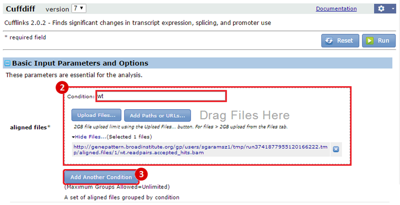
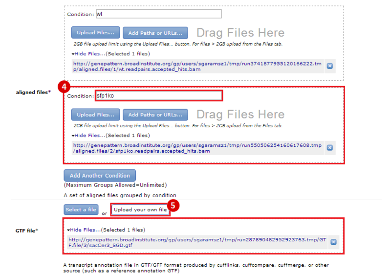
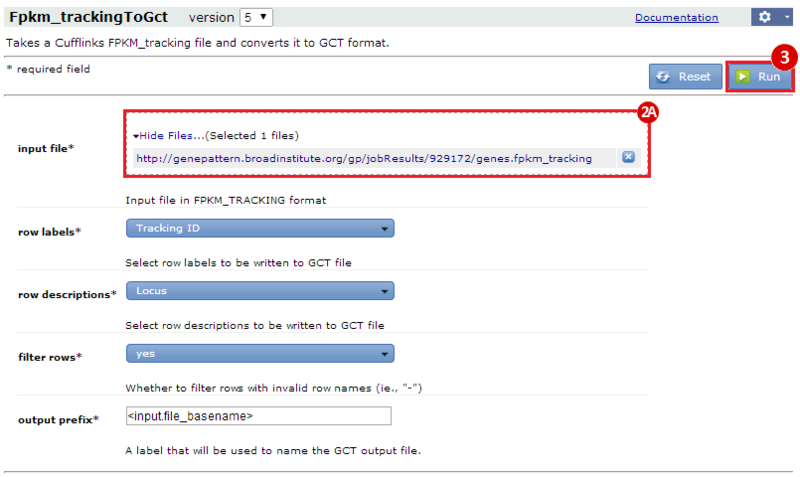
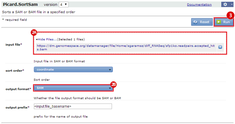
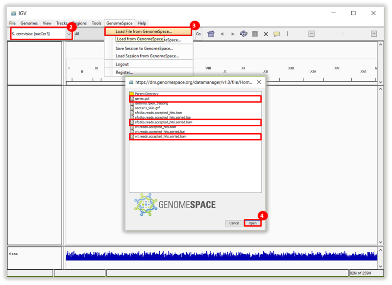
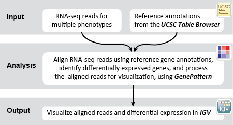
This is an example interpretation of the results from this recipe. First, we used TopHat in GenePattern to align raw reads from RNA-seq to a reference genome (pre-built in Bowtie). After aligning both a wild-type and mutant strain of S. cerevisiae, we used Cufflinks to determine the genes which were differentially expressed when comparing the two phenotypes. We then use IGV to visualize the difference between these two datasets; in particular, we validate that the SFP1KO mutant strain of S. cerevisiae lacks the SFP1 gene.

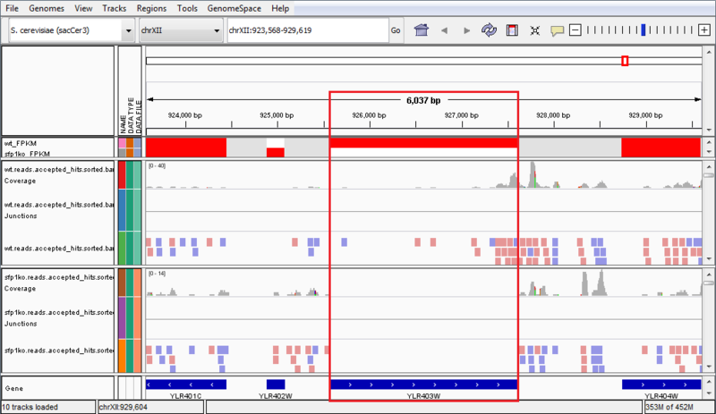
The wt_FPKM track is red in the region of the SFP1 gene, whereas the sfp1ko_FPKM track is white. This is an indicator of gene expression, and shows that the SFP1 gene is not being transcribed in the SFP1KO mutant strain. We can see an additional indicator of this when we compare the wt.reads.accepted_hits.sorted.bam file to the sfp1ko.reads.accepted_hits.sorted.bam file. These are the tracks which have red and blue boxes to indicate where reads aligned against the reference genome. We can see there are several reads aligned in the WT strain to the SFP1 gene, but the area is blank in the SPF1KO mutant, showing that no reads from that gene aligned against the reference genome. These results confirm that the SFP1 gene was knocked-out in the SFP1KO mutant strain of S. cerevisiae. However, the results in this example are not necessarily significant and are only a simple representation of possible results.


Posted by swear0712 on March 04, 2016 01:17

Posted by BrunoBSouzaa on June 30, 2016 16:30

Is GenePattern working ok??? I'm trying to use it but I keep getting an error message... "GenePattern Server error preparing job 1314526 for execution.org.genepattern.server.executor.CommandExecutorException: Error adding job to queue, gpJobNo=1314526, DrmaaException=denied: parallel environment "smp" does not exist job rejected: the requested parallel environment "smp" does not exist" Can someone help me???

Posted by ted on June 30, 2016 16:44

I forwarded your comment to the GenePattern team at gp-help@broadinstitute.org but they could not find your job on the public server. Could you contact them directly to see if they can help sort this out?

Submit a Comment

History