- GenomeSpace Recipes
 GenomeSpace.org
- What is GenomeSpace?
- Tools
- Recipes
- Documentation
- User Guide
Read the detailed guide to the user interface
- Tool Guide
Learn how to access GenomeSpace functionality for each Tool
- FAQ
See answers to frequently asked questions
- Presentations and Videos
Access talks by the GenomeSpace community
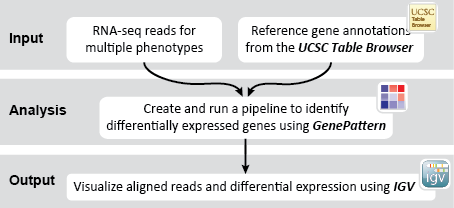
- End-to-End Analyses
Provides description for end-to-end analyses.
- User Guide
- Developers
- Support
- About