Content ucsc gp igv

Identify and visualize expressed transcripts in RNA-seq data

Added by GenomeSpaceTeam on 2015.04.21 Official logo
Last updated on over 3 years ago.


Summary

Which genes are highly expressed, based on my RNA-seq data? Are any of the highly expressed genes also differentially expressed?

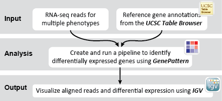
This recipe provides an outline of one method to identify and visualize genes and isoforms that are highly expressed in RNA-seq data. In particular, this recipe utilizes an analysis pipeline, allowing a user to chain together multiple analysis steps into one workflow that can be run in one step. An example use of this recipe is a case where an investigator wants to process several datasets in the same way, in which case the pipeline will allow the investigator to re-use the same modules and parameters, over and over again.


Given a set of raw RNA-seq reads, the goal is to align the reads to a reference genome, estimate expression abundance levels for reference genes and isoforms, filter out low-expressed genes and isoforms, and visualize the read alignments and their expression levels. In particular, this recipe uses the UCSC Table Browser to retrieve a reference genome to align RNA-seq reads against. We also uses several modules in GenePattern to align the reads against the reference genome, and to identify differentially expressed genes when comparing two conditions. Finally, we use IGV to visualize the differentially expressed genes.

Why differential expression analysis? We assume that most genes are not expressed all the time, but rather are expressed in specific tissues, stages of development, or under certain conditions. Genes which are expressed in one condition, such as cancerous tissue, are said to be differentially expressed when compared to normal conditions. To identify which genes change in response to specific conditions (e.g. cancer), we must filter or process the dataset to remove genes which are not informative.


Inputs

To complete this recipe, we will need RNA-seq reads, and reference gene annotations to align the reads against. In this example, we examine human RNA-seq data. The RNA-seq reads are in FASTQ/FASTA >  format, and can be gzipped. We will need the following datasets, which can be downloaded from the GenomeSpace Public folder.

Public  >  RecipeData  >  SequenceData  >  RNA_seq.r1.fastq: this is human RNA-seq data, forward reads.

Public  >  RecipeData  >  SequenceData  >  RNA_seq.r2.fastq: this is human RNA-seq data, reverse reads.

Outputs

Recipe steps

  • UCSC Table Browser
    1. Getting reference gene annotations
  • GenePattern
    1. Creating a pipeline of modules in GenePattern
    2. Running the pipeline
    3. Saving results back to GenomeSpace
  • IGV
    1. Loading data into IGV
    2. Visualizing transcripts

  1. Launch UCSC Table Browser from GenomeSpace by clicking on the icon.
  2. Download the reference gene annotations from UCSC. For the example dataset, enter the following parameters:
    1. clade: Mammal
    2. genome: Human
    3. assembly: Feb. 2009 (GRCh37/hg19)
    4. group: Genes and Gene Predictions
    5. track: UCSC Genes
    6. region: genome
    7. output format: GTF - gene transfer format
    8. Send output to: Select the GenomeSpace checkbox.
    9. output file: Give the output a name. For the example data, we name it UCSC_hg19.gtf.
  3. Click get output to retrieve the file. This will take you to a new page which loads the file to GenomeSpace. The output file should appear in your GenomeSpace home directory.
  4. Optional: close the UCSC Table Browser website.

NOTE: If you have not yet associated your GenomeSpace account with your GenePattern account, you will be asked to do so. If you do not yet have a GenePattern account, you can automatically generate a new account that will be associated with your GenomeSpace account.

Creating a new pipeline

  1. Launch GenePattern from GenomeSpace by clicking on the icon.
  2. Navigate to the Modules & Pipelines tab on the GenePattern toolbar. Do not click; instead, hover your cursor over the tab and click New Pipeline in the drop-down menu to load the Pipeline Designer interface.
  3. OPTIONAL: In the right-hand information panel, change the Pipeline Name to, e.g., RNA_Exp. Other descriptive information (Description, Author, etc.) may be added by the user as desired.

Adding TopHat to the pipeline

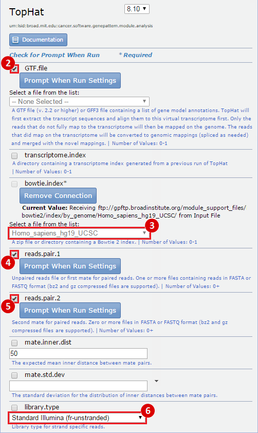
  1. Using either the Search Modules field or the Browse Modules button, select the TopHat module. A purple box titled TopHat will appear in the designer space while the right-hand information panel will change to display TopHat-specific parameters.
  2. Select the GTF.file checkbox.
  3. In the prebuilt.bowtie.index context menu, choose "Homo_sapiens_hg19_UCSC".
  4. Select the reads.pair.1 checkbox.
  5. Select the reads.pair.2 checkbox.
  6. In the library.type context menu, choose "Standard Illumina (fr-unstranded)".

Adding Picard.SortSam to the pipeline

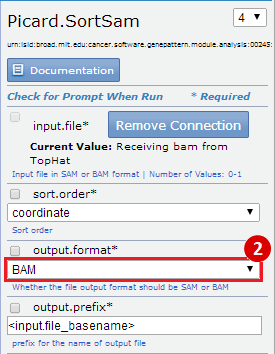
  1. Using either the Search Modules field or the Browse Modules button, select the Picard.SortSam module. A purple box titled Picard.SortSam will appear in the designer space while the right-hand information panel will change to display Picard.SortSam-specific parameters.
  2. In the output.format context menu, choose BAM.

  3. Connect the TopHat and Picard.SortSam modules by clicking on the arrow button in the bottom-right corner of the TopHat box (output) and dragging to the arrow button at the top-left corner of the Picard.SortSam box next to input.file. A purple arrow should appear, connecting the two modules.
  4. Click on the context menu at the bottom of the Picard.SortSam output box and choose bam.

Adding Cufflinks to the pipeline

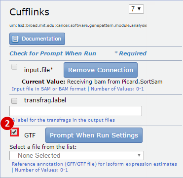
  1. Using either the Search Modules field or the Browse Modules button, select the Cufflinks module. A purple box titled Cufflinks will appear in the designer space while the right-hand information panel will change to display Cufflinks-specific parameters.
  2. Select GTF.file to have the pipeline prompt the user to provide this file when run.

  3. Connect the Picard.SortSam and Cufflinks modules by clicking on the arrow button in the bottom-right corner of the Picard.SortSam box (output) and dragging to the arrow button at the top-left corner of the Cufflinks box next to input.file. A purple arrow should appear, connecting the two modules.
  4. Click on the context menu at the bottom of the Cufflinks output box and choose genes.fpkm_tracking.

Adding Fpkm_trackingToGct to the pipeline

  1. Using either the Search Modules field or the Browse Modules button, select the Fpkm_trackingToGct module. A purple box titled Fpkm_trackingToGct will appear in the designer space while the right-hand information panel will change to display Fpkm_trackingToGct-specific parameters.
  2. Connect the Cufflinks and Fpkm_trackingToGct modules by clicking on the arrow button in the bottom-right corner of the Cufflinks box (output) and dragging to the arrow button at the top-left corner of the Fpkm_trackingToGct box next to input.file. A purple arrow should appear, connecting the two buttons.
  3. Click the Save button to save the pipeline.
  4. Click the Run Pipeline button in the dialog box to run the pipeline.

NOTE: A Pipeline Issues dialog box may appear, displaying warnings found in the pipeline. In the case of our model recipe, these warnings may be ignored.

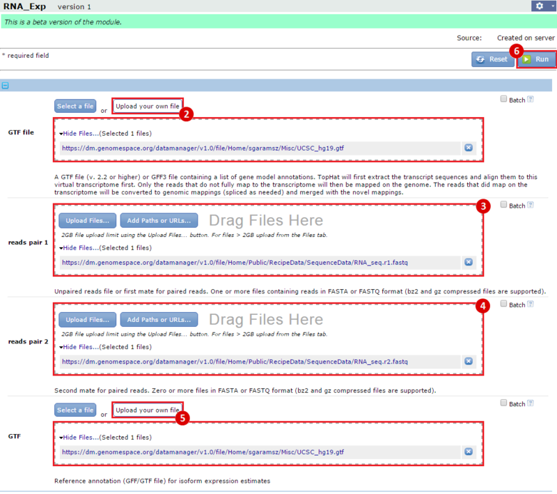
  1. Using the GenomeSpace tab in the GenePattern menu, navigate to the location of your input files. In this example recipe, we will use files RNA_seq.r1.fastq and RNA_seq.r2.fastq.
  2. For the first GTF file parameter, click the Upload your own file button. Navigate to Your Home Directory, then click and drag the GTF file, UCSC_hg19.gtf, to the input box.
  3. Navigate to Public  >  RecipeData  >  SequenceData and drag the first FASTQ file, RNA_seq.r1.fastq, to the reads pair 1 parameter.
  4. Staying in the same folder, drag the second FASTQ file, RNA_seq.r2.fastq, to the reads pair 2 parameter.
  5. For the second GTF file parameter, click the Upload your own file button. Navigate to Your Home Directory, then click and drag the GTF file, UCSC_hg19.gtf, to the input box.
  6. Click Run to submit the pipeline job.

NOTE: It may take several hours to run this pipeline, depending on the size of the files and whether you are using the GenePattern public server.

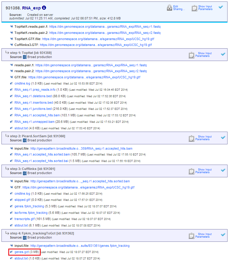
Example output from the pipeline:

  1. Save the following files to GenomeSpace:
    1. TopHat1.reads.pair.1.accepted_hits.sorted.bam
    2. TopHat1.reads.pair.1.accepted_hits.sorted.bai
    3. genes.gct
  2. Use one of the following methods for saving files:
    1. From the job processing view, click the context menu (blue arrow) next to the dataset (e.g., genes.gct), then choose Save to GenomeSpace.
    2. From the Modules & Pipelines start page, navigate to Jobs. Click on the file, then choose Send to GenomeSpace.
  3. OPTIONAL: close GenePattern.

Loading reference data into IGV.

  1. Launch IGV from GenomeSpace by clicking on the context menu and choosing Launch, prompting the download of a .jnlp file. Double-click the file to launch IGV.
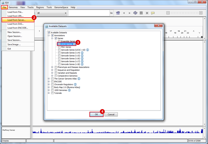
  2. To load a pre-built reference dataset into IGV, navigate to File > Load from Server....
  3. Select the 'UCSC Genes' reference dataset by expanding the following drop-down menus: Annotations > Genes. Choose the UCSC Genes checkbox.
    NOTE: Check only the 'UCSC Genes' box. Checking the 'Genes' or 'Annotations' checkboxes will check all boxes under that heading, i.e., it will load additional datasets that are not needed for this recipe
  4. Click OK to load the dataset.

Loading RNA-seq data into IGV.

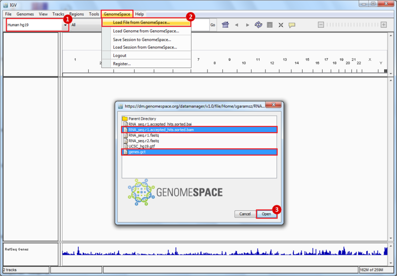
  1. Load a reference genome into IGV by using the IGV genome selection drop-down menu. Make sure the reference genome matches the samples you are using, e.g., H. sapiens samples should use the Human hg19 genome, as in this example.
  2. Use the GenomeSpace tab to import files by clicking on the Load File from GenomeSpace... option.
  3. To load files, navigate to the directory in GenomeSpace which contains the file, then click the file to select it, and then click Open. Load the following files into IGV:
    NOTE: each file is loaded separately
    1. RNA_seq.r1.accepted_hits.sorted.bam
    2. genes.gct


  1. From the GenomeSpace homepage, navigate to and right-click on the genes.gct file. Select Preview from the context menu.
  2. In the preview window, copy a UCSC tracking id (under tracking_id). In this example, we use uc001aal.
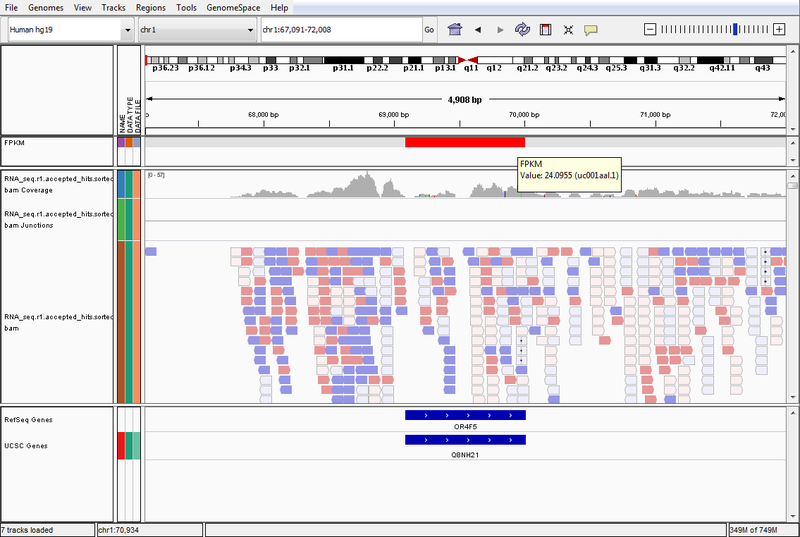
  3. Return to IGV and paste this tracking id into the search bar at the top of the window. Hit enter or click the Go button. A visual representation of the mapped reads will appear.
  4. Display the FPKM values of the transcript by hovering the mouse over FPKM bar.

Results Interpretation

This is an example interpretation of the results from this recipe. First, we used GenePattern to create and run a pipeline which aligned raw reads from RNA-seq to a reference genome (pre-built in Bowtie) using TopHat, then identified differentially expressed genes using Cufflinks. We then used IGV to visualize the FPKM counts of the aligned reads for an example gene, uc001aal.

The wt_FPKM track is red in the region of the uc001aal gene, which indicates a high FPKM count for that gene. If we examine the *.accepted_hits.bam track in IGV, we can see that we have several reads aligning to this particular gene in the genome. However, the results in this example are not necessarily significant and are only a simple representation of possible results.


Submit a Comment

History