Reciperesourcepage3
Recipe workflow

GenomeSpace recipes provide step-by-step instructions for performing integrative bioinformatic data analyses using GenomeSpace tools and data sources. Recipes guide users through common analyses, starting with obtaining input data, followed by analyzing data by passing it to GenomeSpace-enabled tools. In addition, recipes guide users in the interpretation of the results of analyses.

To learn more about recipes, read the Recipe Usage Guide or try browsing recipes!

Community

Check out our F1000 GenomeSpace Channel for published, community-contributed recipes.

F1000

Do you have questions about a recipe? Visit our community forum!

Still have questions? Contact us!

List of All Recipes

Which genes lie in my copy number variation regions? Are there any sets of co-regulated genes in these aberrant regions?

This recipe provides a method for identifying and visualizing a network of co-regulated genes that are associated with aberrant regions identified by single nucleotide polymorphism (SNP) arrays. An example use of this recipe is a case where an investigator may want to find which genes are located in regions that exhibit significant changes (e.g. amplification or deletion) in cancer cells.


This recipe provides one method for identifying and visualizing aberrant regions in Diffuse Large B-Cell Lymphoma (DLBCL) cancer cells. This recipe uses copy-number variation (CNV) data from SNP arrays, and evaluates the expression of aberrant regions using a microarray dataset. Regions that are significantly changed (e.g., amplified or deleted) in cancer cells are defined by the GISTIC algorithm. In particular, this recipe makes use of several Galaxy tools to find the overlap between the aberrant regions and reference genes, and uses GenePattern to process the microarray dataset. Genomica is used to find module networks of co-regulated genes associated with these aberrant regions. A module network is a model which identifies regulatory modules from gene expression data, especially modules of co-regulated genes and their regulators. The module also identifies the conditions under which the regulation can occur.

Why analyze copy number variation regions? Copy number variations (CNVs) are large alterations to genomes, such as duplication or deletion of large segments of a chromosome. These variations in the genome have been associated with different conditions, such as cancer. In this recipe, we explore the scenario in which CNVs are elevated in a cancer cell line, and our goal is to determine the function of these duplicated genes.

Does my gene expression dataset contain a module network of regulatory genes? Does the network have any special features?

This recipe provides one method for creating and visualizing a module network of regulatory genes. An example use of this recipe is a case where an investigator may want to evaulate an expression dataset to find regulatory genes such as transcription factors, and then determine if they are connected in a network.


In particular, the regulatory genes of interest are genes which regulate other genes associated with an embryonic stem cell (ESC) state. This 'stemness signature' is a feature common to ESCs, as well as induced pluripotent stem cells (iPSCs), and also in a compendium of human cancers, such as breast cancer. This recipe recapitulates research by Wong et al., in Cell Stem Cell (2008), "Module map of stem cell genes guides creation of epithelial cancer stem cells."

We use a gene expression dataset of primary human breast cancer tumor samples (described in Chin, K. et al, Cancer Cell, 2006), and create a module network by projecting a set of stemness regulators onto the gene expression dataset, using Genomica. A module network is a model which identifies regulatory modules from gene expression data, especially modules of co-regulated genes and their regulators. The module also identifies the conditions under which the regulation can occur.

After obtaining the module network, we visualize it using Cytoscape. Since the network is very large, we then filter it to just a subnetwork of stemness regulators and their connections, again using Cytoscape. This provides us with a visual representation of the stemness regulators as they appear projected onto a breast cancer tumor dataset.


Does my RNA-Seq data contain noticeable batch effects? Can I remove any batch effects I find?

This recipe provides one method to assess RNA-seq count data for potential batch effects. Identified batch effects are removed using the ComBat algorithm (Johnson, Rabinovic, and Li). An example use case of this recipe is when an investigator wants to correct data and account for confounding variables generated by effects such as using different reagents or processing samples at different times.


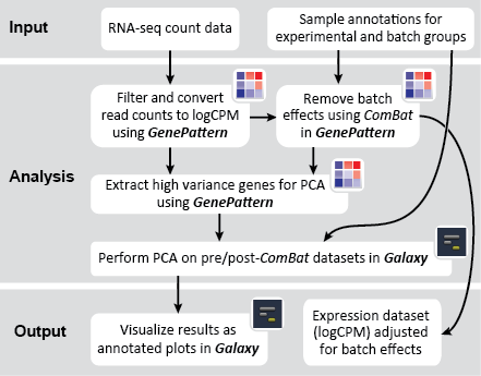
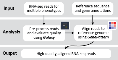
This recipe uses count data and sample annotations derived from two separate RNA-seq experiments and relies upon Principal Component Analysis (PCA) as a primary means of evaluating the dataset for batch effects. In particular, this recipe utilizes a number of GenePattern modules to filter and preprocess the RNA-seq count data and to normalize the dataset using the ComBat algorithm. We then use Galaxy to view the influence of batch effects in our pre- and post-normalization datasets.

Why consider batch effects (a.k.a. confounders)? A "batch" or "confounding" variable can be generally defined as an extraneous variable that may correlate or anti-correlate with our variables of interest. Failing to account for confounding variables or batch effects can lead us to draw spurious conclusions from our data. For example:

Albert is comparing the hardiness of two different E. coli strains, X and Y, by measuring their production of various stress proteins under a mild bactericide. However, Albert's bactericide stock is running low and he ends up using two different stocks of the same bactericide over the course of this experiment. Here, bactericide stock is a confounding or batch variable. Perhaps one bactericide stock is more potent than the other. Albert will need to be careful in how he analyzes his data. He must somehow ensure that differences in stress protein abundances between his X and Y strains are driven by the biological differences of these two strains rather than differences in the bactericide stocks.

Efforts can be undertaken to minimize batch effects by ensuring proper experimental design, e.g., simplifying protocols to eliminate potential confounders. If batches are unavoidable, it is also important to randomize samples across these batches such that differences between batches can be attributed to batch effects rather than biological differences. But despite these efforts, unforeseen batch effects may still be present in any experiment. Thus, we should be aware of the degree to which these unwanted factors influence our results and be prepared to use various statistical methods to remove these unwanted factors if needed.

How do we identify batch effects? There are a variety of methods for identifying batch effects. Sometimes, potential batches can be identified at the outset of a project based on its experimental design. For example, if samples must be processed in separate groups due to the limiting capacity of a sequencer, then these processing groups are likely to introduce batch effects. If batches can be pre-identified, then the scientist can include identical control samples in each batch. Any variation in measurements from these control samples can then be attributed to and used to quantify a batch effect.

Another common method is to visualize data using a PCA projection. PCA uses a linear transformation to transform a dataset into a space of linearly uncorrelated, orthogonal "principal components". More simply, PCA is a way of visualizing data such that underlying structures are revealed. We encourage users to learn more about PCA (Ma and Dai's 2011 article in Briefings in Bioinformatics is a good starting point). By re-projecting with PCA, we can identify those variables, including batch variables, that are contributing to large variances in the dataset.

Which genes are differentially expressed between my two phenotypes, based on my RNA-seq data?

This recipe provides one method to identify differentially expressed genes in RNA-seq read data. An example use of this recipe is a case where an investigator may want to compare two phenotypes, such as two types of cancer, to determine which genes are up- or down-regulated differently between these phenotypes.


In particular, this recipe uses the UCSC Table Browser to retrieve a reference genome to align RNA-seq reads against. We also used several modules in GenePattern to align the reads against the reference genome, and to identify differentially expressed genes when comparing two conditions. Finally, we use IGV to visualize the differentially expressed genes.

Why differential expression analysis? We assume that most genes are not expressed all the time, but rather are expressed in specific tissues, stages of development, or under certain conditions. Genes which are expressed in one condition, such as cancerous tissue, are said to be differentially expressed when compared to normal conditions. To identify which genes change in response to specific conditions (e.g. cancer), we must filter or process the dataset to remove genes which are not informative.


What subnetworks of differentially expressed genes are enriched in my samples? What biological functions are they related to?

This recipe provides a method for identifying differentially expressed genes between two phenotypes, such as tumor and normal, to find subnetworks of interacting proteins and determine their functional annotations. An example use of this recipe is a case where an investigator may want to compare two phenotypes to determine which gene networks are similar between phenotypes, and to determine how functional annotation changes between phenotypes.


In particular, this recipe makes use of several GenePattern modules to identify differentially regulated genes, then uses several Cytoscape plugins to identify potential interactions between gene products, and to visualize the resulting network.

Why differential expression analysis? We assume that most genes are not expressed all the time, but rather are expressed in specific tissues, stages of development, or under certain conditions. Genes which are expressed in one condition, such as cancer tissue, are said to be differentially expressed when compared to normal conditions. To identify which genes change in response to specific conditions (e.g. cancer), we must filter or process the dataset to remove genes which are not informative.

Why protein interaction network analysis? Gene expression analysis results in a list of differentially expressed genes, but it does not explain whether these genes are connected biologically in a pathway or network. To better understanding the underlying biology that drives changes in gene expression analysis, we can perform network analysis to determine whether gene products (e.g. proteins) are reported to interact. To identify potential networks or pathways, we search for highly interconnected subnetworks within a large interaction network.

Which genes are differentially expressed in my microarray data? Are these genes enriched for certain biological pathways?

This recipe provides an outline of one method to identify known biological functions for genes that are differentially expressed between two conditions or phenotypes, using microarray data. An example use of this recipe is a case where an investigator may want to determine if a specific cancer phenotype is associated with expression of certain pathways.


Given a set of differentially expressed genes, the goal is to infer which biological functions (for example, Gene Ontology biological processes) are overrepresented in the set of reference genes found to be differentially expressed. In particular, this recipe uses a gene expression dataset which has two conditions: normal and mild hyperthermia. Then, GenePattern is used to identify differentially expressed genes, and finally MSigDB is used to identify biological functions and pathways that are enriched in the gene set.

Why differential expression analysis? We assume that most genes are not expressed all the time, but rather are expressed in specific tissues, stages of development, or under certain conditions. Genes which are expressed in one condition, such as cancerous tissue, are said to be differentially expressed when compared to normal conditions. To identify which genes change in response to specific conditions (e.g. cancer), we must filter or process the dataset to remove genes which are not informative.

Why perform functional annotation? Many analyses end with the retrieval of a gene list, e.g. gene expression analysis identifies a list of genes which are differentially expressed when comparing multiple conditions. However, often times a researcher has additional questions about the function or relatedness of genes in a gene list: Are the genes a part of the same pathway? Do the gene products interact physically? Do the gene products localize to a specific part of the cell? Are the genes only expressed during a certain stage of development? These questions, and others like them, can be answered by performing functional annotation on gene lists, to better understand the underlying connections between genes.

Do phenotypically different expression datasets share a common signature? Can the signature distinguish phenotypes in an independent dataset?

This recipe provides one method for identifying a consensus gene signature from a training set of several phenotypically distinct gene expression dataset. The recipe then validates the ability of the consensus signature to accurately distinguish phenotypes by using an independent test gene expression dataset. An example use case of this recipe is when an investigator may want to develop a gene expression signature to predict a specific phenotype, such as cancer or another disease.


Background information: What is a consensus gene expression signature?

A gene expression signature is the pattern of expression in a specific group of genes, usually ones that are related by function, position or other biological process. A consensus gene signature is an expression pattern for a specific group of genes, which is shared among different samples or across different phenotypes. For example, a group of genes regulating immune response could be similarly up-regulated during many different, unrelated infections. There are several types of consensus signatures; those that can be derived from gene expression data are called transcriptional consensus signatures. Consensus signatures can be created by overlapping individual gene signatures derived from multiple datasets. Compared to individual gene expression signatures, consensus signatures may be more accurate at distinguishing different phenotypes, such as diseased vs. normal samples.


Use case: Targeting MYCN in Neuroblastoma by BET Bromodomain Inhibition (Puissant et al. , Cancer Discov. 2013).

This study analyzed gene expression data generated from primary neuroblastoma tumors of two genetic classes: tumors harboring MYCN amplification (“MYCN amplified”) and tumors without MYCN amplification (“MYCN non-amplified”). MYCN amplified neuroblastoma is exquisitely dependent on the bromodomain and extra-terminal (BET) family of proteins. As such, treatment of MYCN amplified cell lines or tumors with JQ1, a small-molecule inhibitor of BET proteins, leads to dramatic transcriptional changes and induces cell death.

To identify a consensus signature to predict sensitivity to JQ1 treatment, two training datasets and one test dataset were used. The training dataset included acute myeloid leukemia (AML) and a multiple myeloid leukemia (MM) cell lines, which had been treated with either DMSO (control) or with JQ1 (treatment). The test dataset included MYCN amplified and MYCN nonamplified neuroblastoma primary tumor samples. GenePattern was used to analyze the AML and MM cell lines; for each dataset, a gene expression signature was derived to identify JQ1 response in the cell line. Using Galaxy, the two signatures were then overlapped to determine the consensus signature between the two phenotypes.

GenePattern was used to validate the ability of this JQ1-associated consensus signature to differentiate between phenotypes, by using the signature to hierarchically cluster the test dataset (neuroblastoma). Since the MYCN amplified and MYCN non-amplified neuroblastoma samples should have differing expression profiles, it was hypothesized that the consensus signature would be able to separate the samples by phenotype. Indeed, the consensus signature was able to cluster the MYCN-amplified and MYCN-nonamplified samples separately, revealing that the consensus signature accurately distinguishes the sensitivity-to-JQ1 phenotype.

What coding variants do my exome sequences contain, and are any of them phenotypically interesting?

This recipe provides a method to identify coding variants from exome sequencing data. An example use of this recipe is a case where an investigator may want to identify variants from their alignment data and evaluate the phenotypes.


In particular, this recipe uses the variant detector, FreeBayes, in Galaxy to identify potential variants from short-read alignments and assign them quality scores. We also use other Galaxy tools to pare these potential variants down to a high quality subset and to compare them against a catalog of gold-standard variants. Finally, we use IGV to visualize these variants alongside known pathogenic variants.

Why identify genetic variants? Genetic variants are DNA sequence differences that occur with relative frequency in a population. These variants include single nucleotide polymorphisms (SNPs), insertions and deletions (indels), multi-nucleotide polymorphisms (MNPs), and complex events that are combinations of indels and polymorphisms. With the advent of next generation sequencing technologies, it has become common practice to identify variants using sequence data. This is usually accomplished by comparing sequence data from many samples or individuals against a reference. Identified variants can have many practical applications. For instance, variants that correlate strongly with disease risk may provide insight into the disease's genetic underpinnings. Variants may also be used as biomarkers for disease risk or to DNA "fingerprint" individuals.

Why use exome sequencing data? The human exome comprises all the exonic regions of the human genome. That is, it includes all the DNA sequences that, after transcription into RNA, remain after RNA-splicing, which amounts to about 1% of the entire genome. Whole exome sequencing (WES) thus generates much less data than whole genome sequencing (WGS). Furthermore, since WES focuses almost exclusively on protein-coding regions it is an effective method for identifying coding variants.

NOTE: Working with DNA sequencing data is a computationally and resource intensive process. Files containing raw sequence reads can be many gigabytes in size and can be cumbersome to manage. To maintain the usability of this recipe, we have chosen to work with only a partial region of the human genome, specifically the exonic regions of a chromosome 20.

Which genes are highly expressed, based on my RNA-seq data? Are any of the highly expressed genes also differentially expressed?

This recipe provides an outline of one method to identify and visualize genes and isoforms that are highly expressed in RNA-seq data. In particular, this recipe utilizes an analysis pipeline, allowing a user to chain together multiple analysis steps into one workflow that can be run in one step. An example use of this recipe is a case where an investigator wants to process several datasets in the same way, in which case the pipeline will allow the investigator to re-use the same modules and parameters, over and over again.


Given a set of raw RNA-seq reads, the goal is to align the reads to a reference genome, estimate expression abundance levels for reference genes and isoforms, filter out low-expressed genes and isoforms, and visualize the read alignments and their expression levels. In particular, this recipe uses the UCSC Table Browser to retrieve a reference genome to align RNA-seq reads against. We also uses several modules in GenePattern to align the reads against the reference genome, and to identify differentially expressed genes when comparing two conditions. Finally, we use IGV to visualize the differentially expressed genes.

Why differential expression analysis? We assume that most genes are not expressed all the time, but rather are expressed in specific tissues, stages of development, or under certain conditions. Genes which are expressed in one condition, such as cancerous tissue, are said to be differentially expressed when compared to normal conditions. To identify which genes change in response to specific conditions (e.g. cancer), we must filter or process the dataset to remove genes which are not informative.


Which genes lie in my copy number variation regions? Are these genes enriched for any biological functions or pathways?

This recipe provides a method for identifying biological functions for genes lying in copy number variation (CNV) regions. An example use of this recipe is a case where an investigator may want to examine their list of CNVs to see which genetic regions are amplified or deleted, and determine the biological functions or pathways associated with these amplified or deleted regions.


Copy number variations (CNVs) are large alterations to genomes, such as amplification or deletion of large segments of a chromosome. They can range in size from a focal aberration in a single gene to aberrations covering entire chromosome arms. These variations in the genome have been associated with different conditions, such as cancer. Many genomic analyses produce a set of genes which are assumed to be relevant to an underlying biological mechanism or phenotype. Thus, an investigator often has additional questions about the function or relatedness of these genes: Are they part of the same pathway? Do the gene products interact physically? Do the gene products localize to a specific part of the cell? Are the genes associated with certain stages of development? These questions, and others like them, can be answered by performing functional annotation of gene lists to better understand the underlying connections between genes.

In this particular example, we imagine a scenario in which an investigator identifies CNV regions that are amplified or deleted in glioblastoma multiforme (GBM) tumor samples, using a method called Genomic Identification of Significant Targets in Cancer (GISTIC, Mermel et al. (2011) Genome Biol.). Given a set of CNV regions, the goal is to infer which biological functions (e.g., metabolic and regulatory pathways, chemical perturbation signatures, etc.) are overrepresented in the set of reference genes that overlap with these regions. In particular, this recipe uses several Galaxy tools to find the overlap between CNV regions and reference genes obtained from the UCSC Table Browser. Then it uses the Molecular Signatures Database (MSigDB) to identify biological functions of the overlapped genes.

How can I use this recipe? This recipe may be modified to analyze CNV regions derived from any organism for which an annotated reference genome exists. Nor does the recipe depend on the algorithm used to identify these regions (GISTIC); any source of CNV data can be used. Once an investigator has pinpointed the CNV regions believed to be influencing their phenotype (disease state, cell type, etc.) of study he/she can use this recipe to identify functional pathways that may be affected by these copy number changes and draw closer to an understanding of the mechanisms behind these CNV effects.

Are there specific transcriptional regulators, whose expression and copy number correlate with the expression of genes associated with a specific phenotype?

This recipe provides a method for identifying transcriptional regulators of a gene set associated with a specific phenotype. An example use of this recipe is a case where an investigator may want to identify determine which transcriptional regulators exhibit unique expression phenotypes (e.g. up-regulation or down-regulation). This recipe uses a procedure called "Stepwise Linkage Analysis of Microarray Signatures", first described by Adler et al. (Nat Genetics 2006). This recipe does not use the SLAMS software tool.

In particular, the phenotype is the embryonic stem cell (ESC) state, which is common to ESCs, as well as induced pluripotent stem cells (iPSCs), and also in a compendium of human cancers, such as breast cancer. In this recipe, we are interested in determining which genes transcriptionally regulate this 'stemness signature' of gene expression. This recipe recapitulates research by Wong et al., in Cell Stem Cell (2008), "Module map of stem cell genes guides creation of epithelial cancer stem cells". To recapitulate this research, we will use a procedure called Stepwise Linkage Analysis of Microarray Signatures (SLAMS), which is described by Adler et al. in Nature Genetics (2006), "Genetic regulators of large-scale transcriptional signatures in cancer". A summary description of the SLAMS procedure is listed below, and more information about SLAMS can be found in the review paper, "A SLAMS dunk for cancer regulators", by Kumar-Sinha and Chinnaiyan.

We use a gene expression dataset of primary human breast cancer tumor samples, with a complementary dataset of copy number variation data in array comparative genomic hybridization (aCGH) format, as described in Chin, K. et al, Cancer Cell, 2006. We use a set of stemness signature genes to separate breast cancer tumor samples into those which exhibit the stemness signature and those that do not by creating a module map in Genomica.  A module map characterizes the expression of the gene expression dataset, providing information about sets of genes within the dataset.

We use the classified samples (e.g. stemness signature present vs. stemness signature absent) to normalize the copy number variation data in GenePattern. Next, we identify transcriptional regulators that correlate with the changes in the copy number dataset using a gene set collection from MSigDB, in Genomica. Finally, we identify transcriptional regulators whose amplification or deletion is correlated with up- or downregulation of gene expression. We consider these genes to be 'stemness regulators', i.e. genes which regulate the genes associated with the stemness signature.

Description of the Stepwise Linkage Analysis of Microarray Signatures (SLAMS) procedure (Kumar-Sinha and Chinnaiyan):

  1. Sort tumor samples into groups based on whether the stemness signature is present (“ON”) or absent (“OFF”).
  2. Compare the DNA copy number changes between the groups of tumor samples. Calculate the association between stemness expression and CNV datasets to identify amplifications/deletions associated with the stemness signature.
  3. Select genes which are potential candidate regulators of the stemness signature, based on coordinate gene amplification/deletion and gene expression upregulation/downregulation.
  4. Validate the candidate regulators by assessing their predictive ability in independent samples of tumor samples.

How are SNP-related genes regulated in an expression dataset? Are these genes enriched for particular biological functions?

This recipe provides one method for identifying enriched biological functions in single-nucleotide polymorphisms (SNPs). An example use of this recipe is a case where an investigator may complete a genome-wide association study (GWAS) and wants to know the SNPs that are associated with certain genomic coordinates, in order to determine which genes have particular biological functions.

In this particular example, we imagine a scenario in which an investigator completes a GWAS study, obtaining a list of genomic coordinates that are associated with SNPs. However, simply knowing these genomic coordinates is not always informative; the investigator is also interested in knowing which genes lie in these regions, and what kinds of biological functions these genes may have. In this particular example, we are interested in answering two questions:

  1. Are the genes near these SNPs enriched with particular biological functions?
  2. Are the genes near these SNPs significantly up- or down-regulated in some other biological conditions, such as cancer?

To answer the first question, we will find Gene Ontology functional annotations using Genomica. To answer the second question, we will use the Gene Set Enrichment Analysis (GSEA) module in GenePattern, comparing the SNP-associated genes to a gene expression dataset from a study of epithelial cancer stem cells. This study evaluated the ability of oncogenes to activate an embryonic stem cell program in differentiated adult tumor cells, by transforming human keratinocytes into squamous cell carcinomas using oncogenic Ras and IκBα, plus one of three genes: c-Myc, E2F3, and GFP (Wong et al. 2009. Cell Stem Cell). Comparisons between these three genes showed that c-Myc could re-activate the embroynic stem cell program. Comparing the SNPs to this gene expression dataset can determine whether this set of SNP-associated genes are differentially regulated in c-Myc samples, when compared to other genes such as GFP and E2F3.

What genes are essential to a cell’s survival in a specific environment?

This recipe provides a way to process the results of genome-wide CRISPR-Cas9 knockout screens. In these screens, single guide RNAs (sgRNAs) are designed to bind to and inhibit specific target DNA sequences in genes. Multiple sgRNAs may target the same gene to increase knockout efficiency. In positive screens, essential genes are identified through the sequencing of surviving cells post-selection. The loss of these ‘winning’ genes create cells that are resistant to the selective pressure. In negative screens, essential genes are identified by measuring which genes are lower in abundance post selection. These screens require a non-selected control, which is used to find which genes are essential to survival under the given selective pressures (Miles et al., 2016). Since a large number of sgRNAs can be introduced in a single screen, many genes can be tested for a selection criteria. However, there are many factors to consider in processing of sequenced reads; often multiple sgRNAs in a library target the same gene but with different specificities and efficiencies, and read count distributions vary depending on library and study designs. Additionally, positive selection screens often result in relatively few sgRNAs that dominate the total sequenced reads. The MAGeCK ( Li et al., 2014) method was specifically developed for CRISPR screen analyses with these conditions in mind.

How can we find the molecular mechanism responsible for resistance?

By looking at how the hits in the screen aggregate on an interaction network, we can get an idea of the mechanisms that are essential for the organism to survive an environmental challenge.  The network neighborhood that contains a high concentration of essential genes is strongly implicated as the molecular mechanism by which an organism handles the challenge.

We can find the network neighborhood that is enriched for the screen hits through an algorithm called network propagation (Carlin et al., in press) that is implemented as a feature of the popular network analysis program Cytoscape.  This algorithm will find the closely clustered hits and their network neighbors to build a network diagram of the resistance mechanism.  We can then use GeneMANIA plugin to find enriched terms that easily summarize the biological terms that are enriched in the diagram.

What is Model-based Analysis of Genome-wide CRIPSR/Cas9 Knockout (MAGeCK)?

Model-based Analysis of Genome-wide CRIPSR/Cas9 Knockout (MAGeCK) is an algorithm for identifying both positively and negatively selected sgRNAs and genes from genome-scale CRIPSR/Cas9 knockout screens. The MAGeCK method can be summarized by the following steps:

1. sgRNA read counts are median-ratio normalized.

2. Mean-variance modeling is then used to model each replicate. The statistical significance of each sgRNA is calculated using the learned mean-variance model.

3. Essential genes are determined by looking for genes with consistently highly significant sgRNAs using robust rank aggregation.

Use Case: MAGeCK enables robust identification of essential genes from genome-scale CRISPR/Cas9 knockout screens (Li et al. 2014).

Which genes are differentially expressed between my two phenotypes, based on my RNA-seq data?

This recipe provides one method to identify and visualize gene expression in different diseases and during cell differentiation and development. In collecting ChIP-seq data, we can obtain genome-wide maps of transcription factor occupancies or histone modifications between a treatment and control. In locating these regions, we can integrate ChIP-seq and RNA-seq data to better understand how these binding events regulate associated gene expression of nearby genes. An example use case of this recipe is when Laurent et al. observed how the binding of the Prep1 transcription factor influences gene regulation in mouse embryonic stem cells. The integration of both RNA-seq and Chip-seq data allows a user to identify target genes that are directly regulated by transcription factor binding or any other epigenetic occupancy in the genome.

What is Model-based Analysis of ChiP-seq (MACS)?

Model-based Analysis of ChIP-seq (MACS) is a computational algorithm that identifies genome-wide locations of transcription/chromatin factor binding or histone modifications. It is often preferred over other peak calling algorithms due to its consistency in reporting fewer false positives and its finer spatial resolution. First, it removes redundant reads to account for possible over-amplification of ChIP-DNA, which may affect peak-calling downstream. Then it shifts read positions based on the fragment size distribution to better represent the original ChIP-DNA fragment positions. Once read positions are adjusted, peak enrichment is calculated by identifying regions that are significantly enriched relative to the genomic background. MACS empirically estimates the FDR for experiments with controls for each peak, which can be used as a cutoff to filter enriched peaks. The treatment and control samples are swapped and any enriched peaks found in the control sample are regarded as false positives.

Why differential expression analysis?

We assume that most genes are not expressed all the time, but rather are expressed in specific tissues, stages of development, or under certain conditions. Genes which are expressed in one condition, such as cancerous tissue, are said to be differentially expressed when compared to normal conditions.

Use Case: ChIP-Seq and RNA-Seq Analyses Identify Components of the Wnt and Fgf Signaling Pathways as Prep1 Target Genes in Mouse Embryonic Stem Cells (Laurent et al., PLoS ONE, 2015)

The sample datatset, Series GSE6328, used for this recipe are from NCBI's GEO. We identify the interplay between epigentics and transcriptomics mouse embryonic stems cells by observing how the binding of the transcription factor, Prep1, influences gene expression. Prep1 is predominantly known for its contribution in embryonic development. In comparing genome-wide maps of mouse embryonic cells experiencing Prep1 binding to those that do not, we can identify potential target genes that are being differentially regulated by these binding events.

How do I obtain and analyze data from The Cancer Genome Atlas (TCGA)? Which TCGA datasets have specific mutations in my gene of interest?

This recipe provides a method for identifying and obtaining specific datasets of interest from The Cancer Genome Atlas (TCGA), through a web-based tool called FireBrowse. An example use of this recipe is a case where an investigator may have a gene they are interested in, such as ERCC2, and would like to know if there are mutations in this gene in specific datasets of interest, such as bladder cancer.


Tumors arise from mutational changes to healthy cells, and are frequently deficient in one or more DNA repair pathways. The accumulation of mutations in tumor can be described by the “mutational signature”, a pattern of genetic mutations found in tumor DNA, which reflect different mutation events. Mutational signatures can be specific to certain tissues or cancer types. Many of these mutational signatures are associated with DNA repair pathways.

An in-depth study of urothelial carcinoma, which causes ~150,000 deaths annually, by Kim et al. (Nature Genetics, 2016) has identified a mutational signature in bladder cancer involving the nucleotide-excision repair (NER) pathway. Kim et al. identified a mutational signature involving ERCC2, a gene encoding a DNA helicase which plays a critical role in the NER pathway. Somatic mutations in this gene may prevent proper functioning of the NER pathway, allowing mutations to accumulate. Uniquely, urothelial cancer is the only known tumor type to date in which ERCC2 is significantly mutated.

Kim et al. used the collection of bladder carcinoma (BLCA) samples in The Cancer Genome Atlas (TCGA) to complete their analysis. Data were downloaded from the Broad Institute TCGA Genome Data Analysis Center, and samples were categorized based on mutational status. Tumors with somatic, missense mutations in ERCC2 were compared to non-mutated (wild-type) samples to identify the comprehensive mutational landscape of bladder cancer (also described in this TCGA paper).

This recipe provides a method for processing data from The Cancer Genome Atlas (TCGA), to identify samples which have mutations in specific genes. The purpose of this recipe is to categorize data by mutational status, for further downstream analysis (e.g. comparing tumors of different mutational status, etc.). Data is collected from FireBrowse; Galaxy and GenePattern are used to categorize samples by mutational status and generate GCT and CLS files. The RNA-seq datasets are gene-level normalized RSEM expression estimates.


TCGA Barcodes

The Cancer Genome Atlas labels its datasets with the TCGA barcode, an identifer that describes the metadata associated with sample. You can learn more about the TCGA Barcodes on the NIH National Cancer Institute Wiki page (see also: working with TCGA data).

TCGA barcodes adhere to a certain format: TCGA-00-1111-22A-33B-4444-55. For this recipe, we are interested in the Sample type, indicated by the 22A section of the barcode. For this recipe we are interested in samples with designation 01 (solid tumor, or TP) or 11 (solid tissue normal, or NT), which are paired tumor-normal samples.

What is the quality of my RNA-seq reads? Are my RNA-seq reads of good quality or are there artifacts and errors I should remove and/or be aware of?

This recipe provides an outline of one method to preprocess and determine the quality of RNA-seq libraries. An example use of this recipe is a case where an investigator has completed sequencing of samples, and wants to evaluate and check the quality of the sequencing results before going through the time-consuming process of aligning the reads against a genome.


Given a set of raw RNA-seq reads, the goal is to align the reads to a reference genome and assess the quality of the read alignments by obtaining metrics such as depth of coverage, rRNA contamination, continuity of coverage, and GC bias. The purpose of this recipe is to process raw RNA-seq reads prior to aligning them against a reference genome. In particular, this recipe uses a dataset which has RNA-seq reads contaminated with adapter sequences. First we identify and remove adapter sequences using Galaxy, then we process the data and align it to a reference genome using GenePattern.

Why remove adapter sequences? Adapter sequences are short pieces of DNA with known sequence, which are used to link DNA molecules together. In particular, these are used to link an unknown DNA sequence to a sequencing primer, in order to sequence the unknown DNA strand. Most of the time adapter sequences are removed during pre-processing when data is sent to a researcher; however, sometimes some adapter sequences remain. It is important to remove these sequences before aligning reads to a genome.


This recipe recapitulates research by Pfefferle et al., in Genome Biology(2013), "Transcriptomic classification of genetically engineered mouse models of breast cancer identifies human subtype counterparts", conducted by Charles M Perou's group.  This study encompasses the largest comprehensive genomic dataset to date to identify human-to-mouse disease subtype counterparts, consisting of three independent human breast cancer datasets and 385 DNA gene expression microarrays from 27 GEMMs of mammary carcinoma(Gene Expression Omnibus accession numbers GSE3165, GSE8516, GSE9343, GSE14457, GSE15263, GSE17916, GSE27101, and GSE42640).  In the original study, the similarity between specific human and mouse subtypes was measured using gene set analysis (GSA)(Table 2 in the publication).  To recapitulate this research, we will use Gene Set Enrichment Analysis module(v17) in GenePattern, as an independent method to further validate the research findings.  This effort is supported by NCI Oncology Models Forum(OMF), a collaborative effort to credential cancer mouse models for translational research.

How do I create a custom-generated gene set? Are there any commonalities between custom-generated gene sets, and MSigDB hallmark gene sets?

This recipe provides a method for identifying and visualizing similarities between diverse gene sets relevant to a study. An example use of this recipe is a case where an investigator may want to compare two phenotypes, such as two types of cancer, to determine which gene sets may be similar between these phenotypes.


Background information: What is Gene Set Enrichment Analysis, and why should I use it?

Gene sets are lists of genes that share similar functions, transcriptional regulation, chromosomal positions, pathways, or other biological processes. It is possible to identify gene sets that are enriched or over-represented in a particular phenotype, such as a specific disease. Gene Set Enrichment Analysis (GSEA) is a computational method which determines whether an a priori defined set of genes shows statistically significant, concordant differences between two phenotypes. GSEA can be used with a custom gene set generated by the user, or with the annotated, standardized gene sets which are available in the Molecular Signatures Database (MSigDB) collection. Completing GSEA on a gene expression dataset will identify those gene sets which are significantly enriched in a particular phenotype. Comparing similarities between the top gene sets following GSEA can yield unique insights into the mechanisms associated with a specific phenotype, which cannot be observed using a single-gene analysis.


Use case: Targeting MYCN in Neuroblastoma by BET Bromodomain Inhibition (Puissant et al. , Cancer Discov. 2013).

This study analyzed gene expression data generated from primary neuroblastoma tumors of two genetic classes: tumors harboring MYCN amplification (“MYCN amplified”) and tumors without MYCN amplification (“MYCN non-amplified”). MYCN amplified neuroblastoma is exquisitely dependent on the bromodomain and extra-terminal (BET) family of proteins. As such, treatment of MYCN amplified cell lines or tumors with JQ1, a small-molecule inhibitor of BET proteins, leads to dramatic transcriptional changes and induces cell death.

A training set of gene expression data was analyzed using GenePattern, and custom gene sets were generated representing the MYCN amplified and MYCN non-amplified datasets. The custom-generated gene sets were then concatenated with the Hallmark gene set from MSigDB using tools in Galaxy. Subsequently, a test gene expression dataset of neuroblastoma cell lines treated with JQ1 (treatment) or DMSO (control) was used to rank this collection of gene sets using single-sample Gene Set Enrichment Analysis (ssGSEA).

This analysis reveals that MYCN-associated gene sets are enriched in JQ1-associated datasets, and suggests that JQ1 functions to suppress transcriptional programs mediated by MYCN amplification. The resulting similarities of the top-ranked gene sets are visualized using ConstellationMap, a module available in GenePattern. This helps to highlight similarities and overlaps between gene sets.